This function estimates the posterior distribution for Generalised Additive
Models (GAMs) that can include smooth spline functions, specified in the GAM
formula, as well as latent temporal processes, specified by trend_model.
Further modelling options include State-Space representations to allow covariates and dynamic processes to occur on the latent 'State' level while also capturing observation-level effects. Prior specifications are flexible and explicitly encourage users to apply prior distributions that actually reflect their beliefs.
In addition, model fits can easily be assessed and compared with posterior predictive checks, forecast comparisons and leave-one-out / leave-future-out cross-validation.
Usage
mvgam(
  formula,
  trend_formula,
  knots,
  trend_knots,
  trend_model = "None",
  noncentred = FALSE,
  family = poisson(),
  share_obs_params = FALSE,
  data,
  newdata,
  use_lv = FALSE,
  n_lv,
  trend_map,
  priors,
  run_model = TRUE,
  prior_simulation = FALSE,
  residuals = TRUE,
  return_model_data = FALSE,
  backend = getOption("brms.backend", "cmdstanr"),
  algorithm = getOption("brms.algorithm", "sampling"),
  control = list(max_treedepth = 10, adapt_delta = 0.8),
  chains = 4,
  burnin = 500,
  samples = 500,
  thin = 1,
  parallel = TRUE,
  threads = 1,
  save_all_pars = FALSE,
  silent = 1,
  autoformat = TRUE,
  refit = FALSE,
  lfo = FALSE,
  ...
)
Arguments
- formula
A
formulaobject specifying the GAM observation model formula. These are exactly like the formula for a GLM except that smooth terms,s(),te(),ti(),t2(), as well as time-varyingdynamic()terms, nonparametricgp()terms and offsets usingoffset(), can be added to the right hand side to specify that the linear predictor depends on smooth functions of predictors (or linear functionals of these).In
nmix()family models, theformulais used to set up a linear predictor for the detection probability. Details of the formula syntax used by mvgam can be found inmvgam_formulae- trend_formula
An optional
formulaobject specifying the GAM process model formula. If supplied, a linear predictor will be modelled for the latent trends to capture process model evolution separately from the observation model.Important notes:
Should not have a response variable specified on the left-hand side (e.g.,
~ season + s(year))Use
trendinstead ofseriesfor effects that vary across time seriesIn
nmix()family models, sets up linear predictor for latent abundanceConsider dropping one intercept using
- 1convention to avoid estimation challenges
- knots
An optional
listcontaining user specified knot values for basis construction. For most bases the user simply supplies the knots to be used, which must match up with thekvalue supplied. Different terms can use different numbers of knots, unless they share a covariate.- trend_knots
As for
knotsabove, this is an optionallistof knot values for smooth functions within thetrend_formula.- trend_model
characterorfunctionspecifying the time series dynamics for the latent trend.Available options:
None: No latent trend component (GAM component only, likegam)ZMVNorZMVN(): Zero-Mean Multivariate Normal (Stan only)'RW'orRW(): Random Walk'AR1','AR2','AR3'orAR(p = 1, 2, 3): Autoregressive models'CAR1'orCAR(p = 1): Continuous-time AR (Ornstein–Uhlenbeck process)'VAR1'orVAR(): Vector Autoregressive (Stan only)'PWlogistic','PWlinear'orPW(): Piecewise trends (Stan only)'GP'orGP(): Gaussian Process with squared exponential kernel (Stan only)
Additional features:
Moving average and/or correlated process error terms available for most types (e.g.,
RW(cor = TRUE)for multivariate Random Walk)Hierarchical correlations possible for structured data
See mvgam_trends for details and
ZMVN()for examples
- noncentred
logical. Use non-centred parameterisation for autoregressive trend models? Can improve efficiency by avoiding degeneracies in latent dynamic random effects estimation. Benefits vary by model - highly informative data may perform worse with this option. Available forRW(),AR(),CAR(), ortrend = 'None'withtrend_formula. Not available for moving average or correlated error models.- family
familyspecifying the exponential observation family for the series.Supported families:
gaussian(): Real-valued databetar(): Proportional data on(0,1)lognormal(): Non-negative real-valued datastudent_t(): Real-valued dataGamma(): Non-negative real-valued databernoulli(): Binary datapoisson(): Count data (default)nb(): Overdispersed count databinomial(): Count data with imperfect detection when number of trials is known (usecbind()to bind observations and trials)beta_binomial(): Asbinomial()but allows for overdispersionnmix(): Count data with imperfect detection when number of trials is unknown (State-Space N-Mixture model with Poisson latent states and Binomial observations)
See
mvgam_familiesfor more details.- share_obs_params
logical. IfTRUEand thefamilyhas additional family-specific observation parameters (e.g., variance components, dispersion parameters), these will be shared across all outcome variables. Useful when multiple outcomes share properties. Default isFALSE.- data
A
dataframeorlistcontaining the model response variable and covariates required by the GAMformulaand optionaltrend_formula.Required columns for most models:
series: Afactorindex of the series IDs (number of levels should equal number of unique series labels)time:numericorintegerindex of time points. For most dynamic trend types, time should be measured in discrete, regularly spaced intervals (i.e.,c(1, 2, 3, ...)). Irregular spacing is allowed fortrend_model = CAR(1), but zero intervals are adjusted to1e-12to prevent sampling errors.
Special cases:
Models with hierarchical temporal correlation (e.g.,
AR(gr = region, subgr = species)) should NOT include aseriesidentifierModels without temporal dynamics (
trend_model = 'None'ortrend_model = ZMVN()) don't require atimevariable
- newdata
Optional
dataframeorlistof test data containing the same variables as indata. If included, observations in variableywill be set toNAwhen fitting the model so that posterior simulations can be obtained.- use_lv
logical. IfTRUE, use dynamic factors to estimate series' latent trends in a reduced dimension format. Only available forRW(),AR()andGP()trend models. Default isFALSE. Seelv_correlationsfor examples.- n_lv
integerspecifying the number of latent dynamic factors to use ifuse_lv == TRUE. Cannot exceedn_series. Default ismin(2, floor(n_series / 2)).- trend_map
Optional
data.framespecifying which series should depend on which latent trends. Enables multiple series to depend on the same latent trend process with different observation processes.Required structure:
Column
series: Single unique entry for each series (matching factor levels in data)Column
trend: Integer values indicating which trend each series depends on
Notes:
Sets up latent factor model by enabling
use_lv = TRUEProcess model intercept is NOT automatically suppressed
Not yet supported for continuous time models (
CAR())
- priors
An optional
data.framewith prior definitions or, preferably, a vector ofbrmspriorobjects (seeprior()). Seeget_mvgam_priors()and Details for more information.- run_model
logical. IfFALSE, the model is not fitted but instead the function returns the model file and the data/initial values needed to fit the model outside ofmvgam.- prior_simulation
logical. IfTRUE, no observations are fed to the model, and instead simulations from prior distributions are returned.- residuals
logical. Whether to compute series-level randomized quantile residuals. Default isTRUE. Set toFALSEto save time and reduce object size (can add later using add_residuals).- return_model_data
logical. IfTRUE, the list of data needed to fit the model is returned, along with initial values for smooth and AR parameters, once the model is fitted. Helpful for users who wish to modify the model file to add other stochastic elements. Default isFALSEunlessrun_model == FALSE.- backend
Character string naming the package for Stan model fitting. Options are
"cmdstanr"(default) or"rstan". Can be set globally via"brms.backend"option. See https://mc-stan.org/rstan/ and https://mc-stan.org/cmdstanr/ for details.- algorithm
Character string naming the estimation approach:
"sampling": MCMC (default)"meanfield": Variational inference with factorized normal distributions"fullrank": Variational inference with multivariate normal distribution"laplace": Laplace approximation (cmdstanr only)"pathfinder": Pathfinder algorithm (cmdstanr only)
Can be set globally via
"brms.algorithm"option. Limited testing suggests"meanfield"performs best among non-MCMC approximations for dynamic GAMs.- control
Named
listfor controlling sampler behaviour. Valid elements includemax_treedepth,adapt_deltaandinit.- chains
integerspecifying the number of parallel chains for the model. Ignored for variational inference algorithms.- burnin
integerspecifying the number of warmup iterations to tune sampling algorithms. Ignored for variational inference algorithms.- samples
integerspecifying the number of post-warmup iterations for sampling the posterior distribution.- thin
Thinning interval for monitors. Ignored for variational inference algorithms.
- parallel
logicalspecifying whether to use multiple cores for parallel MCMC simulation. IfTRUE, usesmin(c(chains, parallel::detectCores() - 1))cores.- threads
integer. Experimental option for within-chain parallelisation in Stan usingreduce_sum. Recommended only for experienced Stan users with slow models. Currently works for all families exceptnmix()and when using Cmdstan backend.- save_all_pars
logical. Save draws from all variables defined in Stan'sparametersblock. Default isFALSE.- silent
Verbosity level between
0and2. If1(default), most informational messages are suppressed. If2, even more messages are suppressed. Sampling progress is still printed - setrefresh = 0to disable. Forbackend = "rstan", also setopen_progress = FALSEto prevent additional progress bars.- autoformat
logical. Usestancparser to automatically format Stan code and check for deprecations. For development purposes - leave asTRUE.- refit
logical. Indicates whether this is a refit called usingupdate.mvgam(). Users should leave asFALSE.- lfo
logical. Indicates whether this is part of lfo_cv.mvgam call. Returns lighter model version for speed. Users should leave asFALSE.- ...
Further arguments passed to Stan:
For
backend = "cmdstanr": passed tocmdstanr::sample,cmdstanr::variational,cmdstanr::laplaceorcmdstanr::pathfindermethods
Value
A list object of class mvgam containing model output, the text
representation of the model file, the mgcv model output (for easily generating
simulations at unsampled covariate values), Dunn-Smyth residuals for each
series and key information needed for other functions in the package. See
mvgam-class for details. Use methods(class = "mvgam") for an
overview on available methods.
Details
Dynamic GAMs are useful when we wish to predict future values from time series that show temporal dependence but we do not want to rely on extrapolating from a smooth term (which can sometimes lead to unpredictable and unrealistic behaviours). In addition, smooths can often try to wiggle excessively to capture any autocorrelation that is present in a time series, which exacerbates the problem of forecasting ahead.
As GAMs are very naturally viewed through a Bayesian lens, and we often must model time series that show complex distributional features and missing data, parameters for mvgam models are estimated in a Bayesian framework using Markov Chain Monte Carlo by default.
Getting Started Resources:
General overview:
vignette("mvgam_overview")andvignette("data_in_mvgam")Full list of vignettes:
vignette(package = "mvgam")Real-world examples:
mvgam_use_casesQuick reference: mvgam cheatsheet
Model Specification Details
Formula Syntax: Details of the formula syntax used by mvgam can be
found in mvgam_formulae. Note that it is possible to supply an
empty formula where there are no predictors or intercepts in the observation
model (i.e. y ~ 0 or y ~ -1). In this case, an intercept-only observation
model will be set up but the intercept coefficient will be fixed at zero. This
can be handy if you wish to fit pure State-Space models where the variation in
the dynamic trend controls the average expectation, and/or where intercepts are
non-identifiable (as in piecewise trends).
Families and Link Functions: Details of families supported by mvgam
can be found in mvgam_families.
Trend Models: Details of latent error process models supported by mvgam
can be found in mvgam_trends.
Prior Specifications
Default priors for intercepts and any variance parameters are chosen to be
vaguely informative, but these should always be checked by the user. Prior
distributions for most important model parameters can be altered (see
get_mvgam_priors() for details). Note that latent trends are estimated on
the link scale so choose priors accordingly.
However more control over the model specification can be accomplished by setting
run_model = FALSE and then editing the model code (found in the
model_file slot in the returned object) before running the model using either
rstan or cmdstanr. This is encouraged for complex modelling tasks.
Important: No priors are formally checked to ensure they are in the right syntax so it is up to the user to ensure these are correct.
Model Components
Random Effects: For any smooth terms using the random effect basis
(smooth.construct.re.smooth.spec), a non-centred
parameterisation is automatically employed to avoid degeneracies that are common
in hierarchical models. Note however that centred versions may perform better
for series that are particularly informative, so as with any foray into Bayesian
modelling, it is worth building an understanding of the model's assumptions and
limitations by following a principled workflow. Also note that models are
parameterised using drop.unused.levels = FALSE in jagam
to ensure predictions can be made for all levels of the supplied factor variable.
Observation Level Parameters: When more than one series is included in
data and an observation family that contains more than one parameter is
used, additional observation family parameters (i.e. phi for nb() or sigma
for gaussian()) are by default estimated independently for each series. But if
you wish for the series to share the same observation parameters, set
share_obs_params = TRUE.
Model Diagnostics
Residuals: For each series, randomized quantile (i.e. Dunn-Smyth) residuals are calculated for inspecting model diagnostics. If the fitted model is appropriate then Dunn-Smyth residuals will be standard normal in distribution and no autocorrelation will be evident. When a particular observation is missing, the residual is calculated by comparing independent draws from the model's posterior distribution.
Computational Backend
Using Stan: mvgam is primarily designed to use Hamiltonian Monte Carlo
for parameter estimation via the software Stan (using either the cmdstanr
or rstan interface). There are great advantages when using Stan over Gibbs /
Metropolis Hastings samplers, which includes the option to estimate nonlinear
effects via Hilbert space approximate Gaussian Processes,
the availability of a variety of inference algorithms (i.e. variational inference,
laplacian inference etc...) and capabilities to enforce stationarity for complex Vector Autoregressions.
Because of the many advantages of Stan over JAGS, further development of
the package will only be applied to Stan. This includes the planned addition
of more response distributions, plans to handle zero-inflation, and plans to
incorporate a greater variety of trend models. Users are strongly encouraged to
opt for Stan over JAGS in any proceeding workflows.
Recommended Workflow
How to Start: The mvgam cheatsheet
is a good starting place if you are just learning to use the package. It gives
an overview of the package's key functions and objects, as well as providing a
reasonable workflow that new users can follow.
Recommended Steps:
Data Preparation: Check that your data are in a suitable tidy format for mvgam modeling (see the data formatting vignette for guidance)
Data Exploration: Inspect features of the data using
plot_mvgam_series. Now is also a good time to familiarise yourself with the package's example workflows that are detailed in the vignettes:Model Structure: Carefully think about how to structure linear predictor effects (i.e. smooth terms using
s(),te()orti(), GPs usinggp(), dynamic time-varying effects usingdynamic(), and parametric terms), latent temporal trend components (seemvgam_trends) and the appropriate observation family (seemvgam_families). Useget_mvgam_priors()to see default prior distributions for stochastic parameters.Prior Specification: Change default priors using appropriate prior knowledge (see
prior()). When using State-Space models with atrend_formula, pay particular attention to priors for any variance parameters such as process errors and observation errors. Default priors on these parameters are chosen to be vaguely informative and to avoid zero (using Inverse Gamma priors), but more informative priors will often help with model efficiency and convergence.Model Fitting: Fit the model using either Hamiltonian Monte Carlo or an approximation algorithm (i.e. change the
backendargument) and usesummary.mvgam(),conditional_effects.mvgam(),mcmc_plot.mvgam(),pp_check.mvgam(),pairs.mvgam()andplot.mvgam()to inspect / interrogate the model.Model Comparison: Update the model as needed and use
loo_compare.mvgam()for in-sample model comparisons, or alternatively useforecast.mvgam(),lfo_cv.mvgam()andscore.mvgam_forecast()to compare models based on out-of-sample forecasts (see the forecast evaluation vignette for guidance).Inference and Prediction: When satisfied with the model structure, use
predict.mvgam(),plot_predictions()and/orplot_slopes()for more targeted simulation-based inferences (see "How to interpret and report nonlinear effects from Generalized Additive Models" for some guidance on interpreting GAMs). For time series models, usehindcast.mvgam(),fitted.mvgam(),augment.mvgam()andforecast.mvgam()to inspect posterior hindcast / forecast distributions.Documentation: Use
how_to_cite()to obtain a scaffold methods section (with full references) to begin describing this model in scientific publications.
References
Nicholas J Clark & Konstans Wells (2023). Dynamic generalised additive models (DGAMs) for forecasting discrete ecological time series. Methods in Ecology and Evolution. 14:3, 771-784.
Nicholas J Clark, SK Morgan Ernest, Henry Senyondo, Juniper Simonis, Ethan P White, Glenda M Yenni, KANK Karunarathna (2025). Beyond single-species models: leveraging multispecies forecasts to navigate the dynamics of ecological predictability. PeerJ. 13:e18929 https://doi.org/10.7717/peerj.18929
Examples
# \dontrun{
# =============================================================================
# Basic Multi-Series Time Series Modeling
# =============================================================================
# Simulate three time series that have shared seasonal dynamics,
# independent AR(1) trends, and Poisson observations
set.seed(0)
dat <- sim_mvgam(
T = 80,
n_series = 3,
mu = 2,
trend_model = AR(p = 1),
prop_missing = 0.1,
prop_trend = 0.6
)
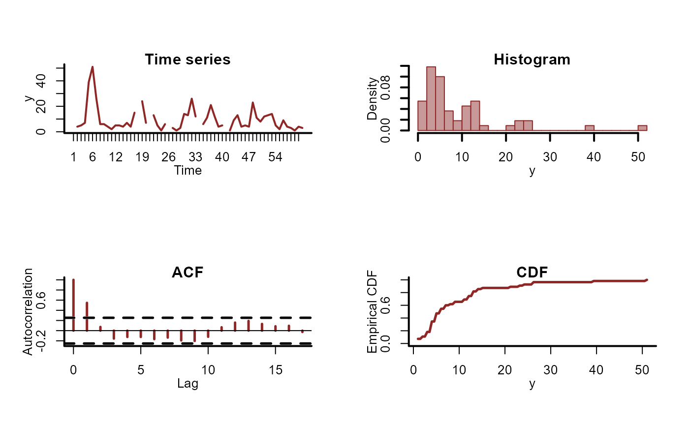
# Plot key summary statistics for a single series
plot_mvgam_series(data = dat$data_train, series = 1)
#> Warning: Removed 5 rows containing non-finite outside the scale range (`stat_bin()`).
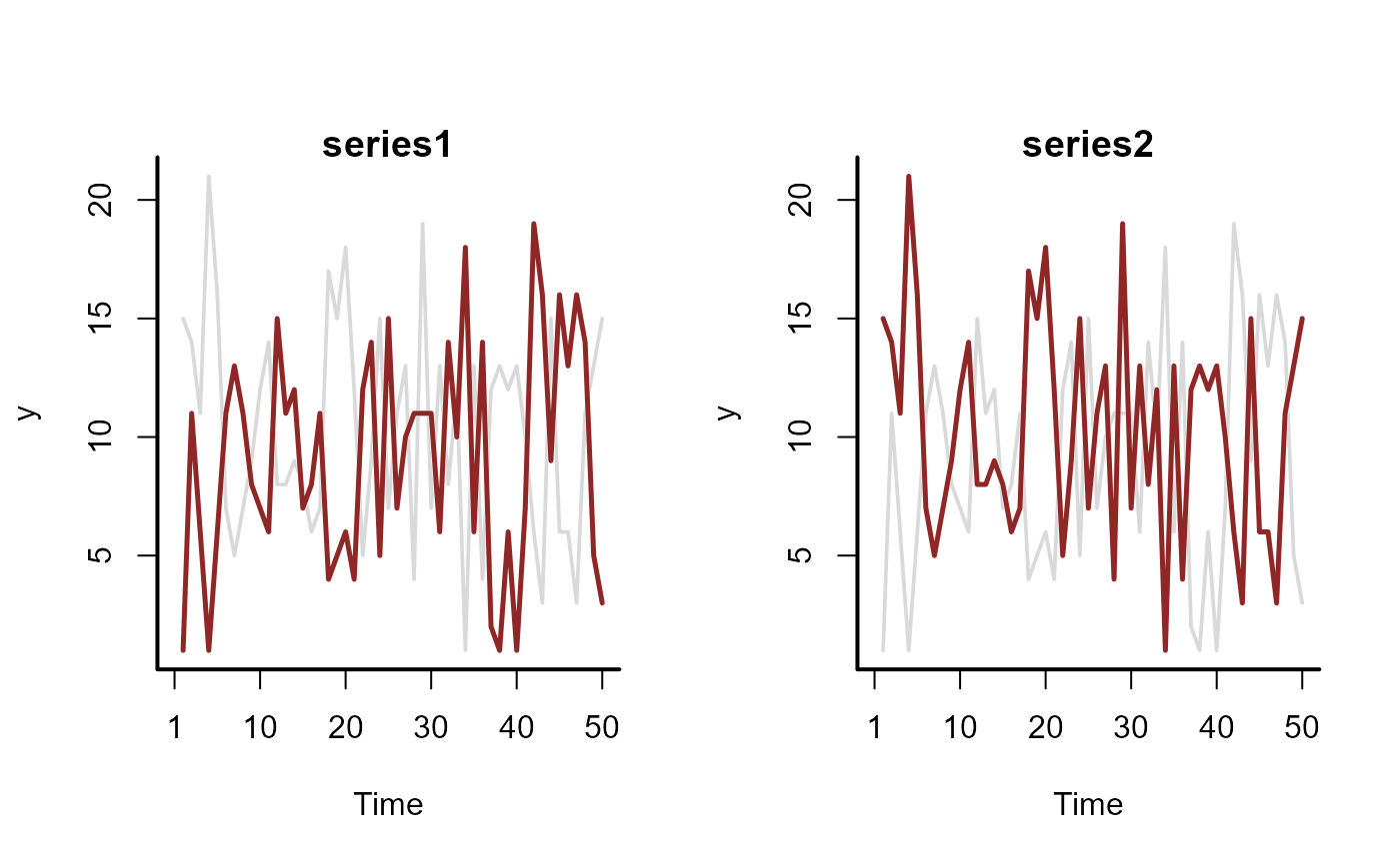
 # Plot all series together
plot_mvgam_series(data = dat$data_train, series = "all")
#> Warning: Removed 2 rows containing missing values or values outside the scale range
#> (`geom_line()`).
# Plot all series together
plot_mvgam_series(data = dat$data_train, series = "all")
#> Warning: Removed 2 rows containing missing values or values outside the scale range
#> (`geom_line()`).
 # Formulate a model using Stan where series share a cyclic smooth for
# seasonality and each series has an independent AR1 temporal process.
# Note that 'noncentred = TRUE' will likely give performance gains.
# Set run_model = FALSE to inspect the returned objects
mod1 <- mvgam(
formula = y ~ s(season, bs = "cc", k = 6),
data = dat$data_train,
trend_model = AR(),
family = poisson(),
noncentred = TRUE,
run_model = FALSE
)
# View the model code in Stan language
stancode(mod1)
#> // Stan model code generated by package mvgam
#> data {
#> int<lower=0> total_obs; // total number of observations
#> int<lower=0> n; // number of timepoints per series
#> int<lower=0> n_sp; // number of smoothing parameters
#> int<lower=0> n_series; // number of series
#> int<lower=0> num_basis; // total number of basis coefficients
#> vector[num_basis] zero; // prior locations for basis coefficients
#> matrix[total_obs, num_basis] X; // mgcv GAM design matrix
#> array[n, n_series] int<lower=0> ytimes; // time-ordered matrix (which col in X belongs to each [time, series] observation?)
#> matrix[4, 4] S1; // mgcv smooth penalty matrix S1
#> int<lower=0> n_nonmissing; // number of nonmissing observations
#> array[n_nonmissing] int<lower=0> flat_ys; // flattened nonmissing observations
#> matrix[n_nonmissing, num_basis] flat_xs; // X values for nonmissing observations
#> array[n_nonmissing] int<lower=0> obs_ind; // indices of nonmissing observations
#> }
#> parameters {
#> // raw basis coefficients
#> vector[num_basis] b_raw;
#>
#> // latent trend AR1 terms
#> vector<lower=-1, upper=1>[n_series] ar1;
#>
#> // latent trend variance parameters
#> vector<lower=0>[n_series] sigma;
#>
#> // raw latent trends
#> matrix[n, n_series] trend_raw;
#>
#> // smoothing parameters
#> vector<lower=0>[n_sp] lambda;
#> }
#> transformed parameters {
#> // basis coefficients
#> vector[num_basis] b;
#>
#> // latent trends
#> matrix[n, n_series] trend;
#> trend = trend_raw .* rep_matrix(sigma', rows(trend_raw));
#> for (s in 1 : n_series) {
#> trend[2 : n, s] += ar1[s] * trend[1 : (n - 1), s];
#> }
#> b[1 : num_basis] = b_raw[1 : num_basis];
#> }
#> model {
#> // prior for (Intercept)...
#> b_raw[1] ~ student_t(3, 1.9, 2.5);
#>
#> // prior for s(season)...
#> b_raw[2 : 5] ~ multi_normal_prec(zero[2 : 5], S1[1 : 4, 1 : 4] * lambda[1]);
#>
#> // priors for AR parameters
#> ar1 ~ std_normal();
#>
#> // priors for smoothing parameters
#> lambda ~ normal(5, 30);
#>
#> // priors for latent trend variance parameters
#> sigma ~ inv_gamma(1.418, 0.452);
#> to_vector(trend_raw) ~ std_normal();
#> {
#> // likelihood functions
#> vector[n_nonmissing] flat_trends;
#> flat_trends = to_vector(trend)[obs_ind];
#> flat_ys ~ poisson_log_glm(append_col(flat_xs, flat_trends), 0.0,
#> append_row(b, 1.0));
#> }
#> }
#> generated quantities {
#> vector[total_obs] eta;
#> matrix[n, n_series] mus;
#> vector[n_sp] rho;
#> vector[n_series] tau;
#> array[n, n_series] int ypred;
#> rho = log(lambda);
#> for (s in 1 : n_series) {
#> tau[s] = pow(sigma[s], -2.0);
#> }
#>
#> // posterior predictions
#> eta = X * b;
#> for (s in 1 : n_series) {
#> mus[1 : n, s] = eta[ytimes[1 : n, s]] + trend[1 : n, s];
#> ypred[1 : n, s] = poisson_log_rng(mus[1 : n, s]);
#> }
#> }
#>
#>
# View the data objects needed to fit the model in Stan
sdata1 <- standata(mod1)
str(sdata1)
#> List of 18
#> $ y : num [1:60, 1:3] 4 5 7 39 51 26 6 6 4 2 ...
#> $ n : int 60
#> $ X : num [1:180, 1:5] 1 1 1 1 1 1 1 1 1 1 ...
#> ..- attr(*, "dimnames")=List of 2
#> .. ..$ : NULL
#> .. ..$ : chr [1:5] "X.Intercept." "V2" "V3" "V4" ...
#> $ S1 : num [1:4, 1:4] 1.244 -0.397 0.384 0.619 -0.397 ...
#> $ zero : num [1:5] 0 0 0 0 0
#> $ p_coefs : Named num 0
#> ..- attr(*, "names")= chr "(Intercept)"
#> $ p_taus : num 0.853
#> $ ytimes : int [1:60, 1:3] 1 4 7 10 13 16 19 22 25 28 ...
#> $ n_series : int 3
#> $ sp : Named num 0.368
#> ..- attr(*, "names")= chr "s(season)"
#> $ y_observed : num [1:60, 1:3] 1 1 1 1 1 1 1 1 1 1 ...
#> $ total_obs : int 180
#> $ num_basis : int 5
#> $ n_sp : num 1
#> $ n_nonmissing: int 164
#> $ obs_ind : int [1:164] 1 2 3 4 5 6 7 8 9 10 ...
#> $ flat_ys : num [1:164] 4 5 7 39 51 26 6 6 4 2 ...
#> $ flat_xs : num [1:164, 1:5] 1 1 1 1 1 1 1 1 1 1 ...
#> ..- attr(*, "dimnames")=List of 2
#> .. ..$ : NULL
#> .. ..$ : chr [1:5] "X.Intercept." "V2" "V3" "V4" ...
#> - attr(*, "trend_model")= chr "AR1"
# Now fit the model
mod1 <- mvgam(
formula = y ~ s(season, bs = "cc", k = 6),
data = dat$data_train,
trend_model = AR(),
family = poisson(),
noncentred = TRUE,
chains = 2,
silent = 2
)
# Extract the model summary
summary(mod1)
#> GAM formula:
#> y ~ s(season, bs = "cc", k = 6)
#> <environment: 0x5582dd828d38>
#>
#> Family:
#> poisson
#>
#> Link function:
#> log
#>
#> Trend model:
#> AR()
#>
#> N series:
#> 3
#>
#> N timepoints:
#> 60
#>
#> Status:
#> Fitted using Stan
#> 2 chains, each with iter = 1000; warmup = 500; thin = 1
#> Total post-warmup draws = 1000
#>
#> GAM coefficient (beta) estimates:
#> 2.5% 50% 97.5% Rhat n_eff
#> (Intercept) 1.900 2.00 2.10 1 602
#> s(season).1 0.073 0.30 0.53 1 744
#> s(season).2 0.580 0.83 1.10 1 531
#> s(season).3 -0.061 0.17 0.39 1 637
#> s(season).4 -0.680 -0.43 -0.20 1 854
#>
#> Approximate significance of GAM smooths:
#> edf Ref.df Chi.sq p-value
#> s(season) 3.664 4 37.54 <2e-16 ***
#> ---
#> Signif. codes: 0 ‘***’ 0.001 ‘**’ 0.01 ‘*’ 0.05 ‘.’ 0.1 ‘ ’ 1
#>
#> standard deviation:
#> 2.5% 50% 97.5% Rhat n_eff
#> sigma[1] 0.41 0.54 0.72 1 410
#> sigma[2] 0.32 0.47 0.65 1 353
#> sigma[3] 0.37 0.50 0.68 1 376
#>
#> precision parameter:
#> 2.5% 50% 97.5% Rhat n_eff
#> tau[1] 2.0 3.5 6.0 1 443
#> tau[2] 2.4 4.5 10.0 1 357
#> tau[3] 2.1 4.0 7.4 1 389
#>
#> autoregressive coef 1:
#> 2.5% 50% 97.5% Rhat n_eff
#> ar1[1] 0.31 0.77 0.990 1.00 297
#> ar1[2] -0.95 -0.46 0.023 1.00 298
#> ar1[3] 0.22 0.71 0.980 1.01 202
#>
#> Stan MCMC diagnostics:
#> ✔ No issues with effective samples per iteration
#> ✔ Rhat looks good for all parameters
#> ✔ No issues with divergences
#> ✔ No issues with maximum tree depth
#>
#> Samples were drawn using sampling(hmc). For each parameter, n_eff is a
#> crude measure of effective sample size, and Rhat is the potential scale
#> reduction factor on split MCMC chains (at convergence, Rhat = 1)
#>
#> Use how_to_cite() to get started describing this model
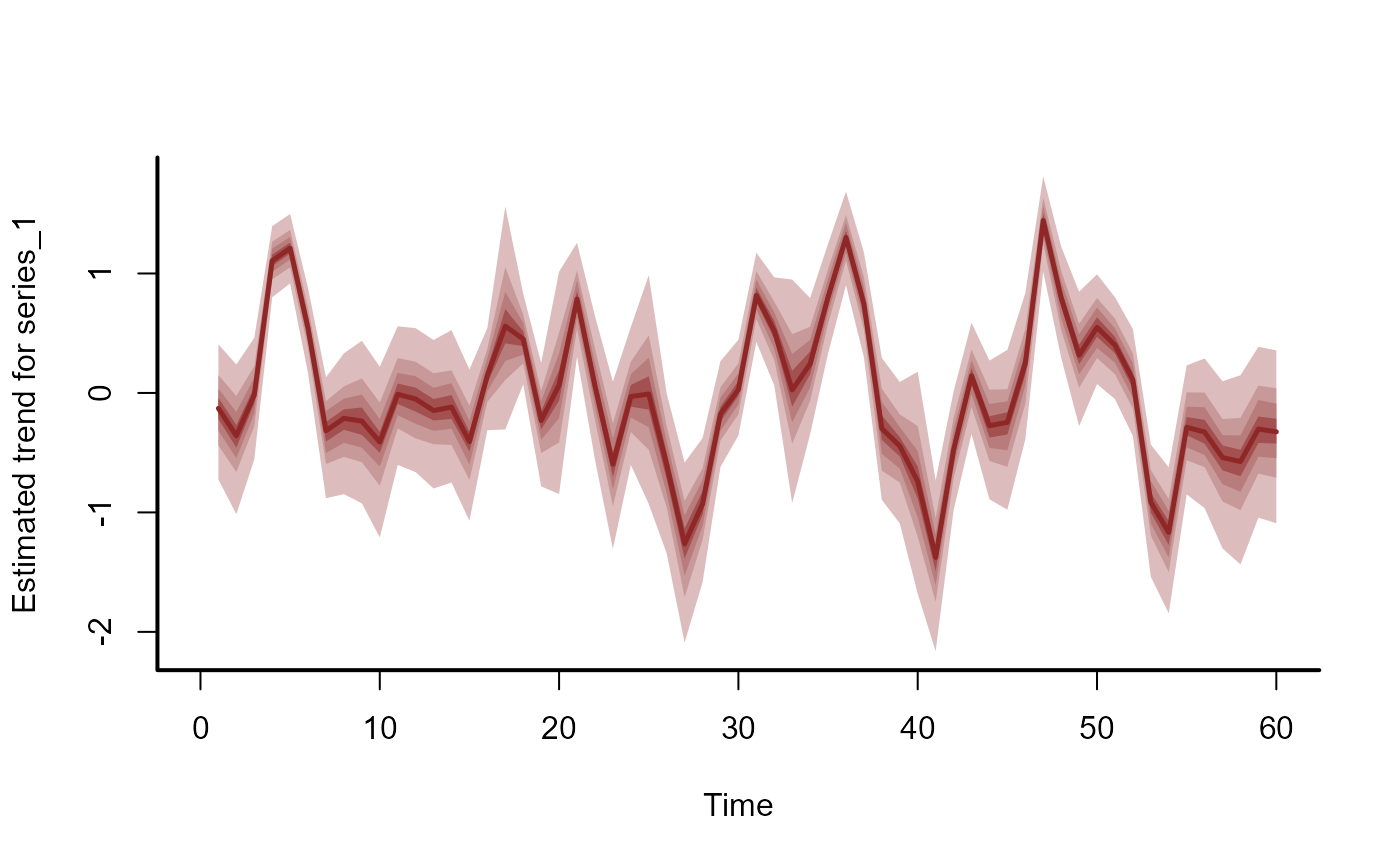
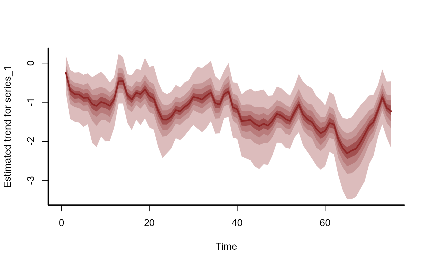
# Plot the historical trend and hindcast distributions for one series
hc_trend <- hindcast(mod1, type = "trend")
plot(hc_trend)
# Formulate a model using Stan where series share a cyclic smooth for
# seasonality and each series has an independent AR1 temporal process.
# Note that 'noncentred = TRUE' will likely give performance gains.
# Set run_model = FALSE to inspect the returned objects
mod1 <- mvgam(
formula = y ~ s(season, bs = "cc", k = 6),
data = dat$data_train,
trend_model = AR(),
family = poisson(),
noncentred = TRUE,
run_model = FALSE
)
# View the model code in Stan language
stancode(mod1)
#> // Stan model code generated by package mvgam
#> data {
#> int<lower=0> total_obs; // total number of observations
#> int<lower=0> n; // number of timepoints per series
#> int<lower=0> n_sp; // number of smoothing parameters
#> int<lower=0> n_series; // number of series
#> int<lower=0> num_basis; // total number of basis coefficients
#> vector[num_basis] zero; // prior locations for basis coefficients
#> matrix[total_obs, num_basis] X; // mgcv GAM design matrix
#> array[n, n_series] int<lower=0> ytimes; // time-ordered matrix (which col in X belongs to each [time, series] observation?)
#> matrix[4, 4] S1; // mgcv smooth penalty matrix S1
#> int<lower=0> n_nonmissing; // number of nonmissing observations
#> array[n_nonmissing] int<lower=0> flat_ys; // flattened nonmissing observations
#> matrix[n_nonmissing, num_basis] flat_xs; // X values for nonmissing observations
#> array[n_nonmissing] int<lower=0> obs_ind; // indices of nonmissing observations
#> }
#> parameters {
#> // raw basis coefficients
#> vector[num_basis] b_raw;
#>
#> // latent trend AR1 terms
#> vector<lower=-1, upper=1>[n_series] ar1;
#>
#> // latent trend variance parameters
#> vector<lower=0>[n_series] sigma;
#>
#> // raw latent trends
#> matrix[n, n_series] trend_raw;
#>
#> // smoothing parameters
#> vector<lower=0>[n_sp] lambda;
#> }
#> transformed parameters {
#> // basis coefficients
#> vector[num_basis] b;
#>
#> // latent trends
#> matrix[n, n_series] trend;
#> trend = trend_raw .* rep_matrix(sigma', rows(trend_raw));
#> for (s in 1 : n_series) {
#> trend[2 : n, s] += ar1[s] * trend[1 : (n - 1), s];
#> }
#> b[1 : num_basis] = b_raw[1 : num_basis];
#> }
#> model {
#> // prior for (Intercept)...
#> b_raw[1] ~ student_t(3, 1.9, 2.5);
#>
#> // prior for s(season)...
#> b_raw[2 : 5] ~ multi_normal_prec(zero[2 : 5], S1[1 : 4, 1 : 4] * lambda[1]);
#>
#> // priors for AR parameters
#> ar1 ~ std_normal();
#>
#> // priors for smoothing parameters
#> lambda ~ normal(5, 30);
#>
#> // priors for latent trend variance parameters
#> sigma ~ inv_gamma(1.418, 0.452);
#> to_vector(trend_raw) ~ std_normal();
#> {
#> // likelihood functions
#> vector[n_nonmissing] flat_trends;
#> flat_trends = to_vector(trend)[obs_ind];
#> flat_ys ~ poisson_log_glm(append_col(flat_xs, flat_trends), 0.0,
#> append_row(b, 1.0));
#> }
#> }
#> generated quantities {
#> vector[total_obs] eta;
#> matrix[n, n_series] mus;
#> vector[n_sp] rho;
#> vector[n_series] tau;
#> array[n, n_series] int ypred;
#> rho = log(lambda);
#> for (s in 1 : n_series) {
#> tau[s] = pow(sigma[s], -2.0);
#> }
#>
#> // posterior predictions
#> eta = X * b;
#> for (s in 1 : n_series) {
#> mus[1 : n, s] = eta[ytimes[1 : n, s]] + trend[1 : n, s];
#> ypred[1 : n, s] = poisson_log_rng(mus[1 : n, s]);
#> }
#> }
#>
#>
# View the data objects needed to fit the model in Stan
sdata1 <- standata(mod1)
str(sdata1)
#> List of 18
#> $ y : num [1:60, 1:3] 4 5 7 39 51 26 6 6 4 2 ...
#> $ n : int 60
#> $ X : num [1:180, 1:5] 1 1 1 1 1 1 1 1 1 1 ...
#> ..- attr(*, "dimnames")=List of 2
#> .. ..$ : NULL
#> .. ..$ : chr [1:5] "X.Intercept." "V2" "V3" "V4" ...
#> $ S1 : num [1:4, 1:4] 1.244 -0.397 0.384 0.619 -0.397 ...
#> $ zero : num [1:5] 0 0 0 0 0
#> $ p_coefs : Named num 0
#> ..- attr(*, "names")= chr "(Intercept)"
#> $ p_taus : num 0.853
#> $ ytimes : int [1:60, 1:3] 1 4 7 10 13 16 19 22 25 28 ...
#> $ n_series : int 3
#> $ sp : Named num 0.368
#> ..- attr(*, "names")= chr "s(season)"
#> $ y_observed : num [1:60, 1:3] 1 1 1 1 1 1 1 1 1 1 ...
#> $ total_obs : int 180
#> $ num_basis : int 5
#> $ n_sp : num 1
#> $ n_nonmissing: int 164
#> $ obs_ind : int [1:164] 1 2 3 4 5 6 7 8 9 10 ...
#> $ flat_ys : num [1:164] 4 5 7 39 51 26 6 6 4 2 ...
#> $ flat_xs : num [1:164, 1:5] 1 1 1 1 1 1 1 1 1 1 ...
#> ..- attr(*, "dimnames")=List of 2
#> .. ..$ : NULL
#> .. ..$ : chr [1:5] "X.Intercept." "V2" "V3" "V4" ...
#> - attr(*, "trend_model")= chr "AR1"
# Now fit the model
mod1 <- mvgam(
formula = y ~ s(season, bs = "cc", k = 6),
data = dat$data_train,
trend_model = AR(),
family = poisson(),
noncentred = TRUE,
chains = 2,
silent = 2
)
# Extract the model summary
summary(mod1)
#> GAM formula:
#> y ~ s(season, bs = "cc", k = 6)
#> <environment: 0x5582dd828d38>
#>
#> Family:
#> poisson
#>
#> Link function:
#> log
#>
#> Trend model:
#> AR()
#>
#> N series:
#> 3
#>
#> N timepoints:
#> 60
#>
#> Status:
#> Fitted using Stan
#> 2 chains, each with iter = 1000; warmup = 500; thin = 1
#> Total post-warmup draws = 1000
#>
#> GAM coefficient (beta) estimates:
#> 2.5% 50% 97.5% Rhat n_eff
#> (Intercept) 1.900 2.00 2.10 1 602
#> s(season).1 0.073 0.30 0.53 1 744
#> s(season).2 0.580 0.83 1.10 1 531
#> s(season).3 -0.061 0.17 0.39 1 637
#> s(season).4 -0.680 -0.43 -0.20 1 854
#>
#> Approximate significance of GAM smooths:
#> edf Ref.df Chi.sq p-value
#> s(season) 3.664 4 37.54 <2e-16 ***
#> ---
#> Signif. codes: 0 ‘***’ 0.001 ‘**’ 0.01 ‘*’ 0.05 ‘.’ 0.1 ‘ ’ 1
#>
#> standard deviation:
#> 2.5% 50% 97.5% Rhat n_eff
#> sigma[1] 0.41 0.54 0.72 1 410
#> sigma[2] 0.32 0.47 0.65 1 353
#> sigma[3] 0.37 0.50 0.68 1 376
#>
#> precision parameter:
#> 2.5% 50% 97.5% Rhat n_eff
#> tau[1] 2.0 3.5 6.0 1 443
#> tau[2] 2.4 4.5 10.0 1 357
#> tau[3] 2.1 4.0 7.4 1 389
#>
#> autoregressive coef 1:
#> 2.5% 50% 97.5% Rhat n_eff
#> ar1[1] 0.31 0.77 0.990 1.00 297
#> ar1[2] -0.95 -0.46 0.023 1.00 298
#> ar1[3] 0.22 0.71 0.980 1.01 202
#>
#> Stan MCMC diagnostics:
#> ✔ No issues with effective samples per iteration
#> ✔ Rhat looks good for all parameters
#> ✔ No issues with divergences
#> ✔ No issues with maximum tree depth
#>
#> Samples were drawn using sampling(hmc). For each parameter, n_eff is a
#> crude measure of effective sample size, and Rhat is the potential scale
#> reduction factor on split MCMC chains (at convergence, Rhat = 1)
#>
#> Use how_to_cite() to get started describing this model
# Plot the historical trend and hindcast distributions for one series
hc_trend <- hindcast(mod1, type = "trend")
plot(hc_trend)
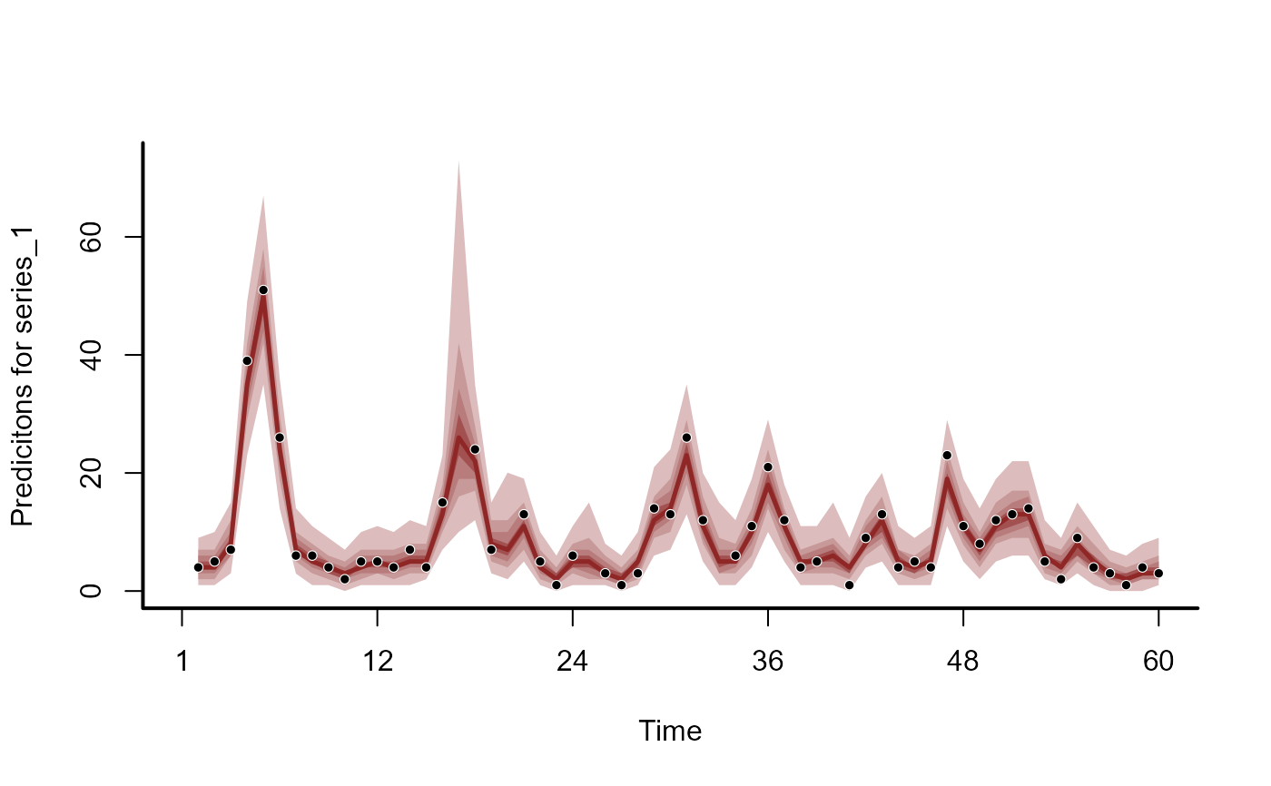
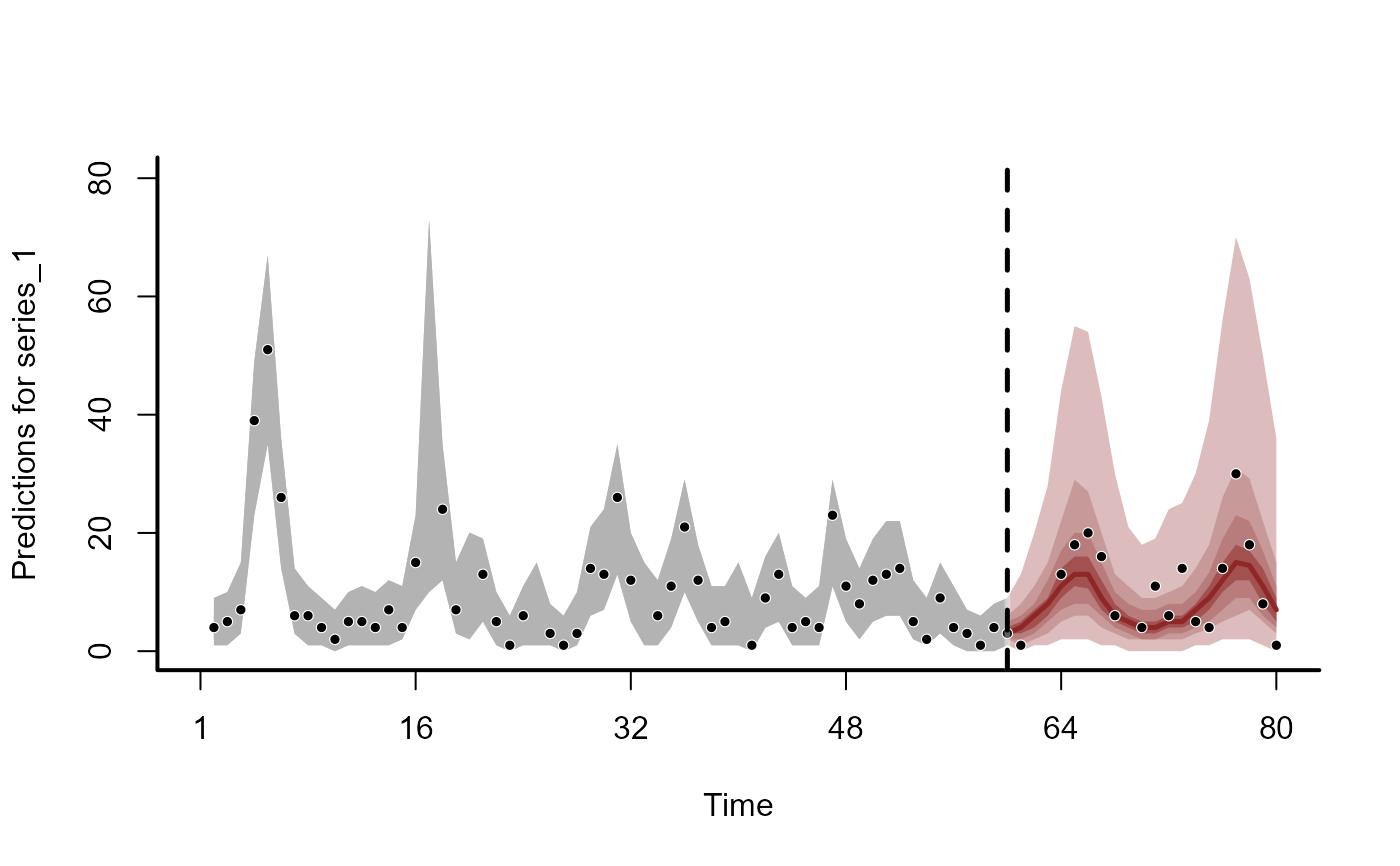
 hc_predicted <- hindcast(mod1, type = "response")
plot(hc_predicted)
#> No non-missing values in test_observations; cannot calculate forecast score
#> Warning: Removed 5 rows containing missing values or values outside the scale range
#> (`geom_point()`).
hc_predicted <- hindcast(mod1, type = "response")
plot(hc_predicted)
#> No non-missing values in test_observations; cannot calculate forecast score
#> Warning: Removed 5 rows containing missing values or values outside the scale range
#> (`geom_point()`).
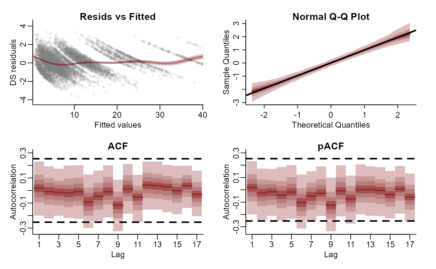
 # Residual diagnostics
plot(mod1, type = "residuals", series = 1)
# Residual diagnostics
plot(mod1, type = "residuals", series = 1)
 resids <- residuals(mod1)
str(resids)
#> num [1:180, 1:4] -0.173 NaN -0.163 0.252 -0.866 ...
#> - attr(*, "dimnames")=List of 2
#> ..$ : NULL
#> ..$ : chr [1:4] "Estimate" "Est.Error" "Q2.5" "Q97.5"
# Fitted values and residuals can be added directly to the training data
augment(mod1)
#> # A tibble: 180 × 14
#> y season year series time .observed .fitted .fit.variability
#> <int> <int> <int> <fct> <int> <int> <dbl> <dbl>
#> 1 4 1 1 series_1 1 4 4.68 1.41
#> 2 NA 1 1 series_2 1 NA 6.98 3.75
#> 3 4 1 1 series_3 1 4 4.68 1.66
#> 4 5 2 1 series_1 2 5 4.76 1.49
#> 5 2 2 1 series_2 2 2 3.87 1.40
#> 6 NA 2 1 series_3 2 NA 5.30 2.91
#> 7 7 3 1 series_1 3 7 8.67 2.39
#> 8 12 3 1 series_2 3 12 11.4 2.94
#> 9 4 3 1 series_3 3 4 5.44 1.85
#> 10 39 4 1 series_1 4 39 36.2 5.75
#> # ℹ 170 more rows
#> # ℹ 6 more variables: .fit.cred.low <dbl>, .fit.cred.high <dbl>, .resid <dbl>,
#> # .resid.variability <dbl>, .resid.cred.low <dbl>, .resid.cred.high <dbl>
# Compute the forecast using covariate information in data_test
fc <- forecast(mod1, newdata = dat$data_test)
str(fc)
#> List of 16
#> $ call :Class 'formula' language y ~ s(season, bs = "cc", k = 6)
#> .. ..- attr(*, ".Environment")=<environment: 0x5582dd828d38>
#> $ trend_call : NULL
#> $ family : chr "poisson"
#> $ family_pars : NULL
#> $ trend_model :List of 7
#> ..$ trend_model: chr "AR1"
#> ..$ ma : logi FALSE
#> ..$ cor : logi FALSE
#> ..$ unit : chr "time"
#> ..$ gr : chr "NA"
#> ..$ subgr : chr "series"
#> ..$ label : language AR()
#> ..- attr(*, "class")= chr "mvgam_trend"
#> ..- attr(*, "param_info")=List of 2
#> .. ..$ param_names: chr [1:8] "trend" "tau" "sigma" "ar1" ...
#> .. ..$ labels : chr [1:8] "trend_estimates" "precision_parameter" "standard_deviation" "autoregressive_coef_1" ...
#> $ drift : logi FALSE
#> $ use_lv : logi FALSE
#> $ fit_engine : chr "stan"
#> $ type : chr "response"
#> $ series_names : Factor w/ 3 levels "series_1","series_2",..: 1 2 3
#> $ train_observations:List of 3
#> ..$ series_1: int [1:60] 4 5 7 39 51 26 6 6 4 2 ...
#> ..$ series_2: int [1:60] NA 2 12 16 6 31 9 15 5 3 ...
#> ..$ series_3: int [1:60] 4 NA 4 NA NA 16 7 7 3 NA ...
#> $ train_times :List of 3
#> ..$ series_1: int [1:60] 1 2 3 4 5 6 7 8 9 10 ...
#> ..$ series_2: int [1:60] 1 2 3 4 5 6 7 8 9 10 ...
#> ..$ series_3: int [1:60] 1 2 3 4 5 6 7 8 9 10 ...
#> $ test_observations :List of 3
#> ..$ series_1: int [1:20] 1 NA NA 13 18 20 16 6 NA 4 ...
#> ..$ series_2: int [1:20] 4 36 8 6 7 NA NA 1 6 4 ...
#> ..$ series_3: int [1:20] 6 8 5 5 19 14 1 1 7 0 ...
#> $ test_times :List of 3
#> ..$ series_1: int [1:20] 61 62 63 64 65 66 67 68 69 70 ...
#> ..$ series_2: int [1:20] 61 62 63 64 65 66 67 68 69 70 ...
#> ..$ series_3: int [1:20] 61 62 63 64 65 66 67 68 69 70 ...
#> $ hindcasts :List of 3
#> ..$ series_1: num [1:1000, 1:60] 3 4 6 4 6 8 2 3 2 2 ...
#> .. ..- attr(*, "dimnames")=List of 2
#> .. .. ..$ : NULL
#> .. .. ..$ : chr [1:60] "ypred[1,1]" "ypred[2,1]" "ypred[3,1]" "ypred[4,1]" ...
#> ..$ series_2: num [1:1000, 1:60] 7 4 5 2 5 9 14 23 4 8 ...
#> .. ..- attr(*, "dimnames")=List of 2
#> .. .. ..$ : NULL
#> .. .. ..$ : chr [1:60] "ypred[1,2]" "ypred[2,2]" "ypred[3,2]" "ypred[4,2]" ...
#> ..$ series_3: num [1:1000, 1:60] 7 0 6 2 4 3 5 13 5 1 ...
#> .. ..- attr(*, "dimnames")=List of 2
#> .. .. ..$ : NULL
#> .. .. ..$ : chr [1:60] "ypred[1,3]" "ypred[2,3]" "ypred[3,3]" "ypred[4,3]" ...
#> $ forecasts :List of 3
#> ..$ series_1: int [1:1000, 1:20] 2 10 10 6 9 7 3 1 5 8 ...
#> ..$ series_2: int [1:1000, 1:20] 0 17 4 6 3 7 11 12 18 11 ...
#> ..$ series_3: int [1:1000, 1:20] 14 4 4 15 14 8 5 14 11 6 ...
#> - attr(*, "class")= chr "mvgam_forecast"
fc_summary <- summary(fc)
head(fc_summary, 12)
#> # A tibble: 12 × 7
#> series time predQ50 predQ2.5 predQ97.5 truth type
#> <fct> <int> <dbl> <dbl> <dbl> <int> <chr>
#> 1 series_1 1 4 1 10 4 response
#> 2 series_1 2 4 1 10 5 response
#> 3 series_1 3 8 3 17 7 response
#> 4 series_1 4 36 22 53 39 response
#> 5 series_1 5 49 31 70.0 51 response
#> 6 series_1 6 24 13.0 38 26 response
#> 7 series_1 7 7 2 16 6 response
#> 8 series_1 8 5 1 12.0 6 response
#> 9 series_1 9 4 0 10 4 response
#> 10 series_1 10 3 0 8 2 response
#> 11 series_1 11 4 0 12 5 response
#> 12 series_1 12 5 1 11 5 response
plot(fc)
#> Out of sample DRPS:
#> 58.499299
#> Warning: Removed 8 rows containing missing values or values outside the scale range
#> (`geom_point()`).
resids <- residuals(mod1)
str(resids)
#> num [1:180, 1:4] -0.173 NaN -0.163 0.252 -0.866 ...
#> - attr(*, "dimnames")=List of 2
#> ..$ : NULL
#> ..$ : chr [1:4] "Estimate" "Est.Error" "Q2.5" "Q97.5"
# Fitted values and residuals can be added directly to the training data
augment(mod1)
#> # A tibble: 180 × 14
#> y season year series time .observed .fitted .fit.variability
#> <int> <int> <int> <fct> <int> <int> <dbl> <dbl>
#> 1 4 1 1 series_1 1 4 4.68 1.41
#> 2 NA 1 1 series_2 1 NA 6.98 3.75
#> 3 4 1 1 series_3 1 4 4.68 1.66
#> 4 5 2 1 series_1 2 5 4.76 1.49
#> 5 2 2 1 series_2 2 2 3.87 1.40
#> 6 NA 2 1 series_3 2 NA 5.30 2.91
#> 7 7 3 1 series_1 3 7 8.67 2.39
#> 8 12 3 1 series_2 3 12 11.4 2.94
#> 9 4 3 1 series_3 3 4 5.44 1.85
#> 10 39 4 1 series_1 4 39 36.2 5.75
#> # ℹ 170 more rows
#> # ℹ 6 more variables: .fit.cred.low <dbl>, .fit.cred.high <dbl>, .resid <dbl>,
#> # .resid.variability <dbl>, .resid.cred.low <dbl>, .resid.cred.high <dbl>
# Compute the forecast using covariate information in data_test
fc <- forecast(mod1, newdata = dat$data_test)
str(fc)
#> List of 16
#> $ call :Class 'formula' language y ~ s(season, bs = "cc", k = 6)
#> .. ..- attr(*, ".Environment")=<environment: 0x5582dd828d38>
#> $ trend_call : NULL
#> $ family : chr "poisson"
#> $ family_pars : NULL
#> $ trend_model :List of 7
#> ..$ trend_model: chr "AR1"
#> ..$ ma : logi FALSE
#> ..$ cor : logi FALSE
#> ..$ unit : chr "time"
#> ..$ gr : chr "NA"
#> ..$ subgr : chr "series"
#> ..$ label : language AR()
#> ..- attr(*, "class")= chr "mvgam_trend"
#> ..- attr(*, "param_info")=List of 2
#> .. ..$ param_names: chr [1:8] "trend" "tau" "sigma" "ar1" ...
#> .. ..$ labels : chr [1:8] "trend_estimates" "precision_parameter" "standard_deviation" "autoregressive_coef_1" ...
#> $ drift : logi FALSE
#> $ use_lv : logi FALSE
#> $ fit_engine : chr "stan"
#> $ type : chr "response"
#> $ series_names : Factor w/ 3 levels "series_1","series_2",..: 1 2 3
#> $ train_observations:List of 3
#> ..$ series_1: int [1:60] 4 5 7 39 51 26 6 6 4 2 ...
#> ..$ series_2: int [1:60] NA 2 12 16 6 31 9 15 5 3 ...
#> ..$ series_3: int [1:60] 4 NA 4 NA NA 16 7 7 3 NA ...
#> $ train_times :List of 3
#> ..$ series_1: int [1:60] 1 2 3 4 5 6 7 8 9 10 ...
#> ..$ series_2: int [1:60] 1 2 3 4 5 6 7 8 9 10 ...
#> ..$ series_3: int [1:60] 1 2 3 4 5 6 7 8 9 10 ...
#> $ test_observations :List of 3
#> ..$ series_1: int [1:20] 1 NA NA 13 18 20 16 6 NA 4 ...
#> ..$ series_2: int [1:20] 4 36 8 6 7 NA NA 1 6 4 ...
#> ..$ series_3: int [1:20] 6 8 5 5 19 14 1 1 7 0 ...
#> $ test_times :List of 3
#> ..$ series_1: int [1:20] 61 62 63 64 65 66 67 68 69 70 ...
#> ..$ series_2: int [1:20] 61 62 63 64 65 66 67 68 69 70 ...
#> ..$ series_3: int [1:20] 61 62 63 64 65 66 67 68 69 70 ...
#> $ hindcasts :List of 3
#> ..$ series_1: num [1:1000, 1:60] 3 4 6 4 6 8 2 3 2 2 ...
#> .. ..- attr(*, "dimnames")=List of 2
#> .. .. ..$ : NULL
#> .. .. ..$ : chr [1:60] "ypred[1,1]" "ypred[2,1]" "ypred[3,1]" "ypred[4,1]" ...
#> ..$ series_2: num [1:1000, 1:60] 7 4 5 2 5 9 14 23 4 8 ...
#> .. ..- attr(*, "dimnames")=List of 2
#> .. .. ..$ : NULL
#> .. .. ..$ : chr [1:60] "ypred[1,2]" "ypred[2,2]" "ypred[3,2]" "ypred[4,2]" ...
#> ..$ series_3: num [1:1000, 1:60] 7 0 6 2 4 3 5 13 5 1 ...
#> .. ..- attr(*, "dimnames")=List of 2
#> .. .. ..$ : NULL
#> .. .. ..$ : chr [1:60] "ypred[1,3]" "ypred[2,3]" "ypred[3,3]" "ypred[4,3]" ...
#> $ forecasts :List of 3
#> ..$ series_1: int [1:1000, 1:20] 2 10 10 6 9 7 3 1 5 8 ...
#> ..$ series_2: int [1:1000, 1:20] 0 17 4 6 3 7 11 12 18 11 ...
#> ..$ series_3: int [1:1000, 1:20] 14 4 4 15 14 8 5 14 11 6 ...
#> - attr(*, "class")= chr "mvgam_forecast"
fc_summary <- summary(fc)
head(fc_summary, 12)
#> # A tibble: 12 × 7
#> series time predQ50 predQ2.5 predQ97.5 truth type
#> <fct> <int> <dbl> <dbl> <dbl> <int> <chr>
#> 1 series_1 1 4 1 10 4 response
#> 2 series_1 2 4 1 10 5 response
#> 3 series_1 3 8 3 17 7 response
#> 4 series_1 4 36 22 53 39 response
#> 5 series_1 5 49 31 70.0 51 response
#> 6 series_1 6 24 13.0 38 26 response
#> 7 series_1 7 7 2 16 6 response
#> 8 series_1 8 5 1 12.0 6 response
#> 9 series_1 9 4 0 10 4 response
#> 10 series_1 10 3 0 8 2 response
#> 11 series_1 11 4 0 12 5 response
#> 12 series_1 12 5 1 11 5 response
plot(fc)
#> Out of sample DRPS:
#> 58.499299
#> Warning: Removed 8 rows containing missing values or values outside the scale range
#> (`geom_point()`).
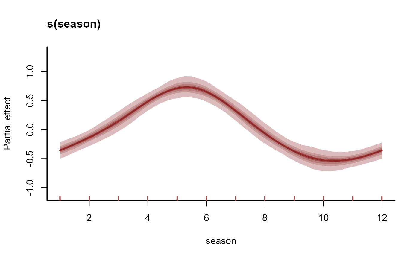
 # Plot the estimated seasonal smooth function
plot(mod1, type = "smooths")
# Plot the estimated seasonal smooth function
plot(mod1, type = "smooths")
 # Plot estimated first derivatives of the smooth
plot(mod1, type = "smooths", derivatives = TRUE)
# Plot estimated first derivatives of the smooth
plot(mod1, type = "smooths", derivatives = TRUE)
 # Plot partial residuals of the smooth
plot(mod1, type = "smooths", residuals = TRUE)
# Plot partial residuals of the smooth
plot(mod1, type = "smooths", residuals = TRUE)
 # Plot posterior realisations for the smooth
plot(mod1, type = "smooths", realisations = TRUE)
# Plot posterior realisations for the smooth
plot(mod1, type = "smooths", realisations = TRUE)
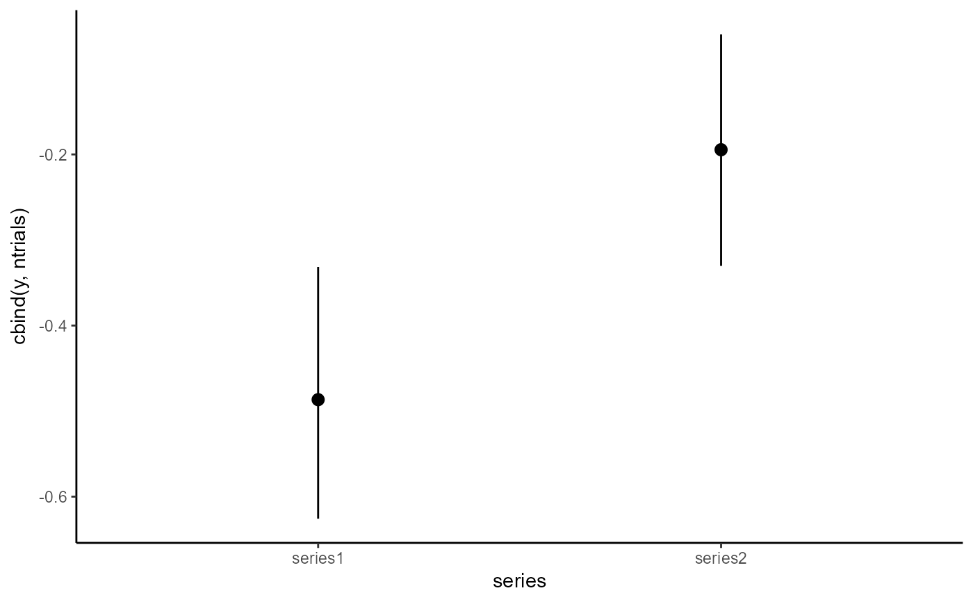
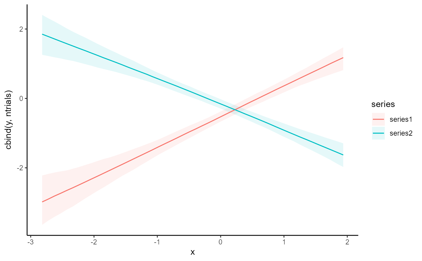
 # Plot conditional response predictions using marginaleffects
conditional_effects(mod1)
# Plot conditional response predictions using marginaleffects
conditional_effects(mod1)
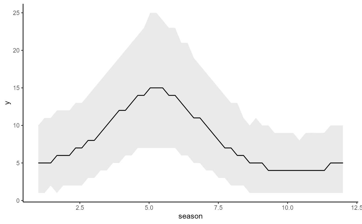 plot_predictions(mod1, condition = "season", points = 0.5)
#> Warning: Removed 16 rows containing missing values or values outside the scale range
#> (`geom_point()`).
plot_predictions(mod1, condition = "season", points = 0.5)
#> Warning: Removed 16 rows containing missing values or values outside the scale range
#> (`geom_point()`).
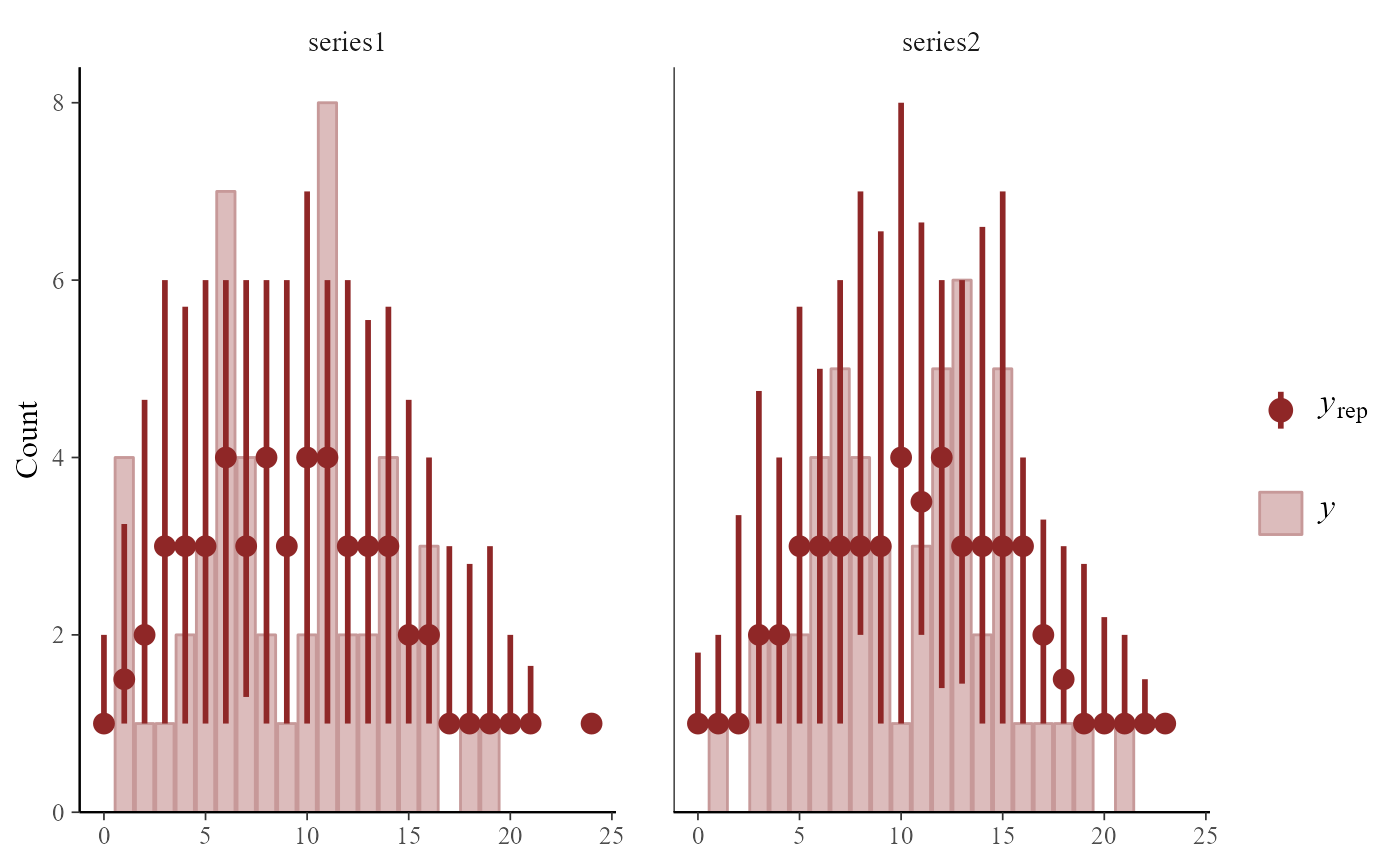
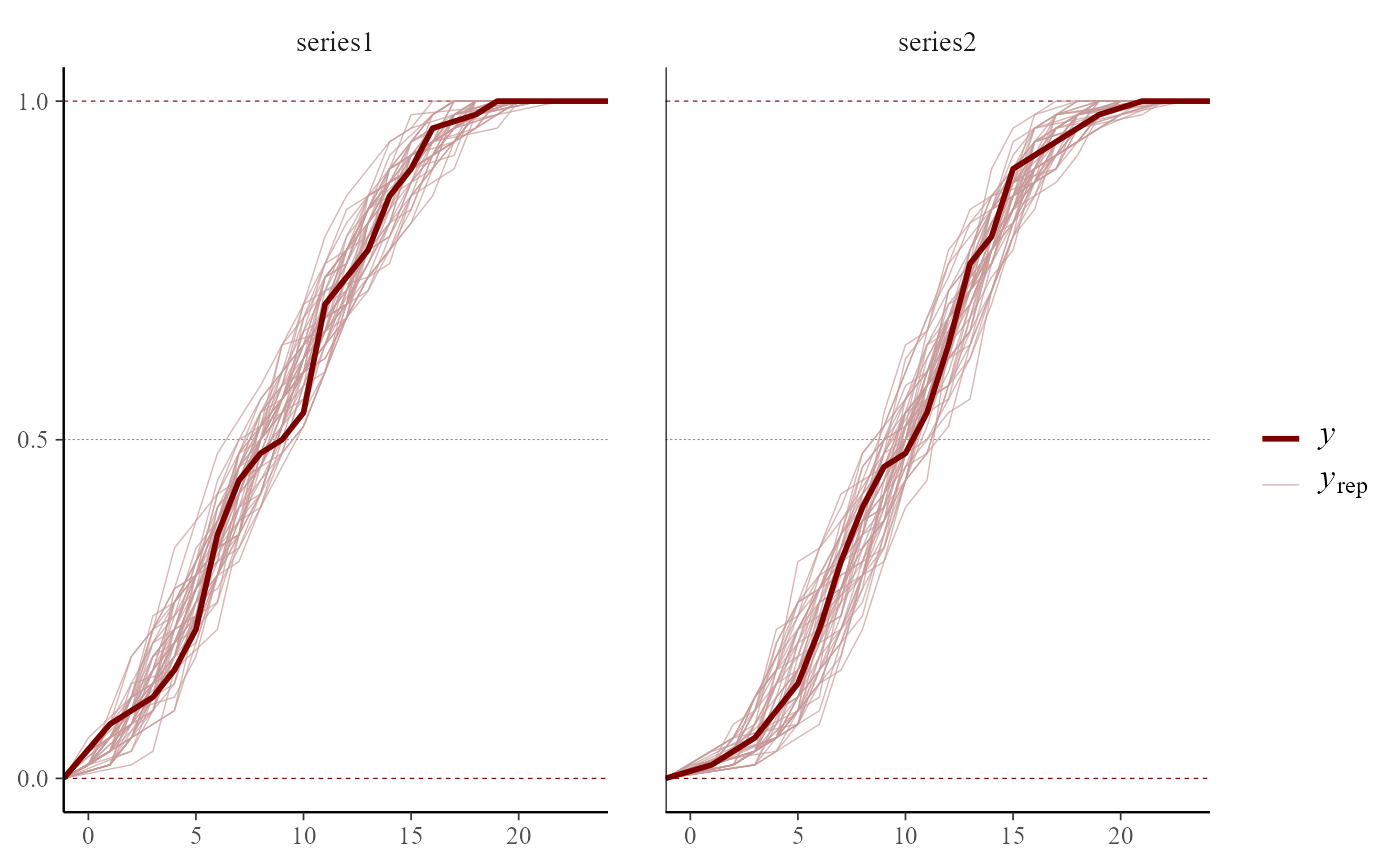
 # Generate posterior predictive checks using bayesplot
pp_check(mod1)
#> Using 10 posterior draws for ppc type 'dens_overlay' by default.
#> Warning: NA responses are not shown in 'pp_check'.
# Generate posterior predictive checks using bayesplot
pp_check(mod1)
#> Using 10 posterior draws for ppc type 'dens_overlay' by default.
#> Warning: NA responses are not shown in 'pp_check'.
 # Extract observation model beta coefficient draws as a data.frame
beta_draws_df <- as.data.frame(mod1, variable = "betas")
head(beta_draws_df)
#> (Intercept) s(season).1 s(season).2 s(season).3 s(season).4
#> 1 1.940875 0.4137472 0.8598868 0.2378396 -0.4088210
#> 2 1.942460 0.3595631 0.8336334 0.1979749 -0.3940571
#> 3 2.017848 0.4184636 0.8373215 -0.1520581 -0.6574271
#> 4 1.927537 0.6949739 0.9827827 0.1354921 -0.2827903
#> 5 2.045359 0.4093142 1.0094558 0.1985756 -0.3792462
#> 6 2.020427 0.4169547 0.9777476 0.1536283 -0.3889246
str(beta_draws_df)
#> 'data.frame': 1000 obs. of 5 variables:
#> $ (Intercept): num 1.94 1.94 2.02 1.93 2.05 ...
#> $ s(season).1: num 0.414 0.36 0.418 0.695 0.409 ...
#> $ s(season).2: num 0.86 0.834 0.837 0.983 1.009 ...
#> $ s(season).3: num 0.238 0.198 -0.152 0.135 0.199 ...
#> $ s(season).4: num -0.409 -0.394 -0.657 -0.283 -0.379 ...
# Investigate model fit
mc.cores.def <- getOption("mc.cores")
options(mc.cores = 1)
loo(mod1)
#> Replacing NAs in `r_eff` with 1s
#> Warning: Some Pareto k diagnostic values are too high. See help('pareto-k-diagnostic') for details.
#>
#> Computed from 1000 by 164 log-likelihood matrix.
#>
#> Estimate SE
#> elpd_loo -817.8 98.2
#> p_loo 136.7 36.0
#> looic 1635.7 196.4
#> ------
#> MCSE of elpd_loo is NA.
#> MCSE and ESS estimates assume MCMC draws (r_eff in [0.4, 1.0]).
#>
#> Pareto k diagnostic values:
#> Count Pct. Min. ESS
#> (-Inf, 0.67] (good) 150 91.5% 45
#> (0.67, 1] (bad) 10 6.1% <NA>
#> (1, Inf) (very bad) 4 2.4% <NA>
#> See help('pareto-k-diagnostic') for details.
options(mc.cores = mc.cores.def)
# =============================================================================
# Vector Autoregressive (VAR) Models
# =============================================================================
# Fit a model to the portal time series that uses a latent
# Vector Autoregression of order 1
mod <- mvgam(
formula = captures ~ -1,
trend_formula = ~ trend,
trend_model = VAR(cor = TRUE),
family = poisson(),
data = portal_data,
chains = 2,
silent = 2
)
# Plot the autoregressive coefficient distributions;
# use 'dir = "v"' to arrange the order of facets correctly
mcmc_plot(
mod,
variable = 'A',
regex = TRUE,
type = 'hist',
facet_args = list(dir = 'v')
)
#> `stat_bin()` using `bins = 30`. Pick better value `binwidth`.
# Extract observation model beta coefficient draws as a data.frame
beta_draws_df <- as.data.frame(mod1, variable = "betas")
head(beta_draws_df)
#> (Intercept) s(season).1 s(season).2 s(season).3 s(season).4
#> 1 1.940875 0.4137472 0.8598868 0.2378396 -0.4088210
#> 2 1.942460 0.3595631 0.8336334 0.1979749 -0.3940571
#> 3 2.017848 0.4184636 0.8373215 -0.1520581 -0.6574271
#> 4 1.927537 0.6949739 0.9827827 0.1354921 -0.2827903
#> 5 2.045359 0.4093142 1.0094558 0.1985756 -0.3792462
#> 6 2.020427 0.4169547 0.9777476 0.1536283 -0.3889246
str(beta_draws_df)
#> 'data.frame': 1000 obs. of 5 variables:
#> $ (Intercept): num 1.94 1.94 2.02 1.93 2.05 ...
#> $ s(season).1: num 0.414 0.36 0.418 0.695 0.409 ...
#> $ s(season).2: num 0.86 0.834 0.837 0.983 1.009 ...
#> $ s(season).3: num 0.238 0.198 -0.152 0.135 0.199 ...
#> $ s(season).4: num -0.409 -0.394 -0.657 -0.283 -0.379 ...
# Investigate model fit
mc.cores.def <- getOption("mc.cores")
options(mc.cores = 1)
loo(mod1)
#> Replacing NAs in `r_eff` with 1s
#> Warning: Some Pareto k diagnostic values are too high. See help('pareto-k-diagnostic') for details.
#>
#> Computed from 1000 by 164 log-likelihood matrix.
#>
#> Estimate SE
#> elpd_loo -817.8 98.2
#> p_loo 136.7 36.0
#> looic 1635.7 196.4
#> ------
#> MCSE of elpd_loo is NA.
#> MCSE and ESS estimates assume MCMC draws (r_eff in [0.4, 1.0]).
#>
#> Pareto k diagnostic values:
#> Count Pct. Min. ESS
#> (-Inf, 0.67] (good) 150 91.5% 45
#> (0.67, 1] (bad) 10 6.1% <NA>
#> (1, Inf) (very bad) 4 2.4% <NA>
#> See help('pareto-k-diagnostic') for details.
options(mc.cores = mc.cores.def)
# =============================================================================
# Vector Autoregressive (VAR) Models
# =============================================================================
# Fit a model to the portal time series that uses a latent
# Vector Autoregression of order 1
mod <- mvgam(
formula = captures ~ -1,
trend_formula = ~ trend,
trend_model = VAR(cor = TRUE),
family = poisson(),
data = portal_data,
chains = 2,
silent = 2
)
# Plot the autoregressive coefficient distributions;
# use 'dir = "v"' to arrange the order of facets correctly
mcmc_plot(
mod,
variable = 'A',
regex = TRUE,
type = 'hist',
facet_args = list(dir = 'v')
)
#> `stat_bin()` using `bins = 30`. Pick better value `binwidth`.
 # Plot the process error variance-covariance matrix in the same way
mcmc_plot(
mod,
variable = 'Sigma',
regex = TRUE,
type = 'hist',
facet_args = list(dir = 'v')
)
#> `stat_bin()` using `bins = 30`. Pick better value `binwidth`.
# Plot the process error variance-covariance matrix in the same way
mcmc_plot(
mod,
variable = 'Sigma',
regex = TRUE,
type = 'hist',
facet_args = list(dir = 'v')
)
#> `stat_bin()` using `bins = 30`. Pick better value `binwidth`.
 # Calculate Generalized Impulse Response Functions for each series
irfs <- irf(
mod,
h = 12,
cumulative = FALSE
)
# Plot some of them
plot(irfs, series = 1)
# Calculate Generalized Impulse Response Functions for each series
irfs <- irf(
mod,
h = 12,
cumulative = FALSE
)
# Plot some of them
plot(irfs, series = 1)
 plot(irfs, series = 2)
 # Calculate forecast error variance decompositions for each series
fevds <- fevd(mod, h = 12)
# Plot median contributions to forecast error variance
plot(fevds)
# Calculate forecast error variance decompositions for each series
fevds <- fevd(mod, h = 12)
# Plot median contributions to forecast error variance
plot(fevds)
 # =============================================================================
# Dynamic Factor Models
# =============================================================================
# Now fit a model that uses two RW dynamic factors to model
# the temporal dynamics of the four rodent species
mod <- mvgam(
captures ~ series,
trend_model = RW(),
use_lv = TRUE,
n_lv = 2,
data = portal_data,
chains = 2,
silent = 2
)
#> Warning in '/tmp/Rtmpz9mhjG/model_fe1a9373f4bc428a5906ce7b23b30b3c.stan', line 20, column 31 to column 48:
#> Found int division:
#> n_lv * (n_lv - 1) / 2
#> Values will be rounded towards zero. If rounding is not desired you can
#> write the division as
#> n_lv * (n_lv - 1) / 2.0
#> If rounding is intended please use the integer division operator %/%.
#> Warning in '/tmp/Rtmpz9mhjG/model-2112108f99c1.stan', line 20, column 33 to column 50:
#> Found int division:
#> n_lv * (n_lv - 1) / 2
#> Values will be rounded towards zero. If rounding is not desired you can
#> write the division as
#> n_lv * (n_lv - 1) / 2.0
#> If rounding is intended please use the integer division operator %/%.
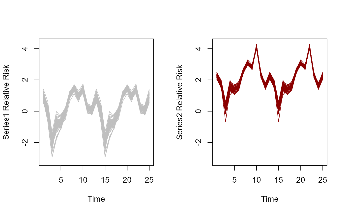
# Plot the factors
plot(mod, type = 'factors')
# =============================================================================
# Dynamic Factor Models
# =============================================================================
# Now fit a model that uses two RW dynamic factors to model
# the temporal dynamics of the four rodent species
mod <- mvgam(
captures ~ series,
trend_model = RW(),
use_lv = TRUE,
n_lv = 2,
data = portal_data,
chains = 2,
silent = 2
)
#> Warning in '/tmp/Rtmpz9mhjG/model_fe1a9373f4bc428a5906ce7b23b30b3c.stan', line 20, column 31 to column 48:
#> Found int division:
#> n_lv * (n_lv - 1) / 2
#> Values will be rounded towards zero. If rounding is not desired you can
#> write the division as
#> n_lv * (n_lv - 1) / 2.0
#> If rounding is intended please use the integer division operator %/%.
#> Warning in '/tmp/Rtmpz9mhjG/model-2112108f99c1.stan', line 20, column 33 to column 50:
#> Found int division:
#> n_lv * (n_lv - 1) / 2
#> Values will be rounded towards zero. If rounding is not desired you can
#> write the division as
#> n_lv * (n_lv - 1) / 2.0
#> If rounding is intended please use the integer division operator %/%.
# Plot the factors
plot(mod, type = 'factors')
 #> # A tibble: 2 × 2
#> Factor Contribution
#> <chr> <dbl>
#> 1 Factor 1 0.531
#> 2 Factor 2 0.469
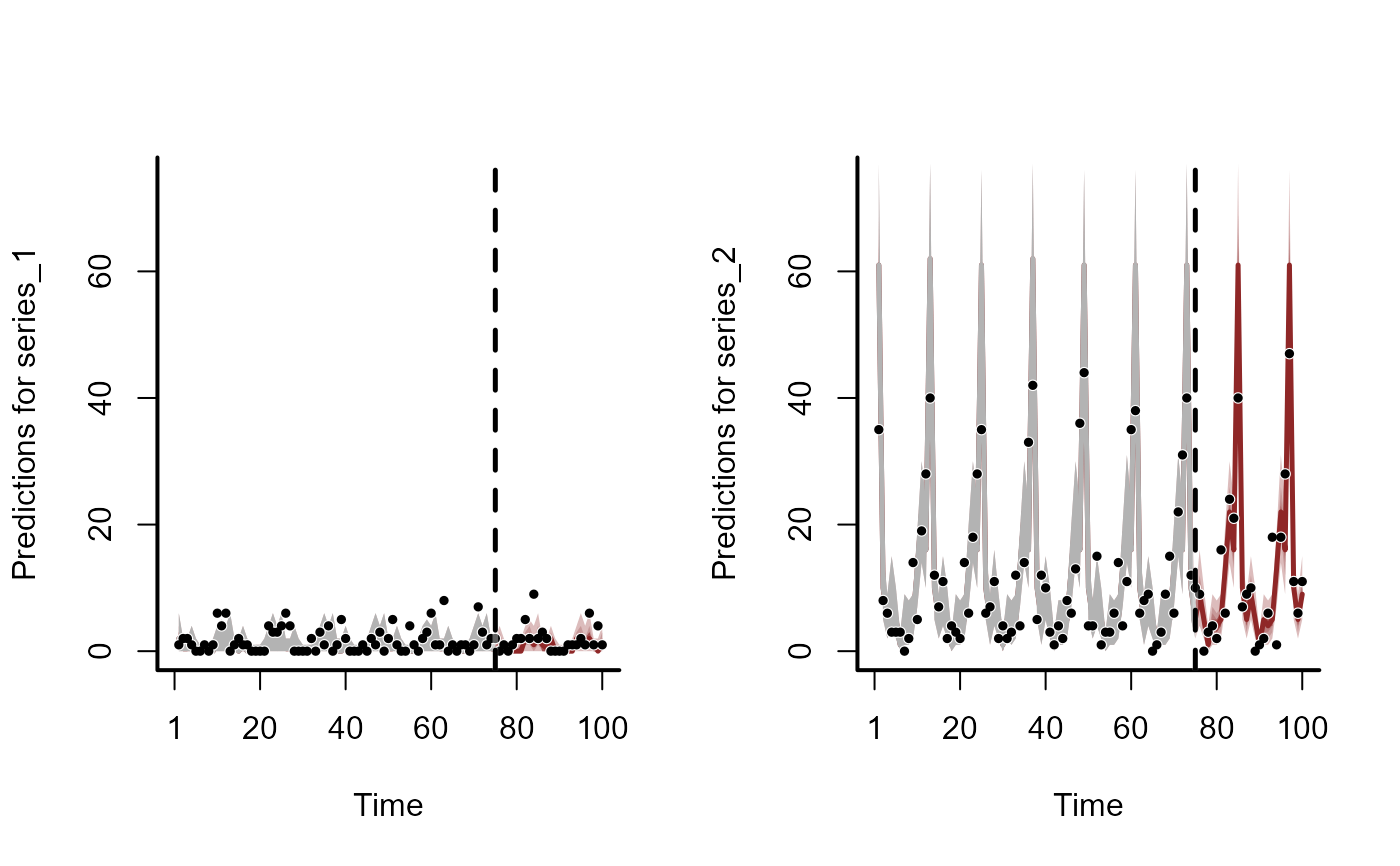
# Plot the hindcast distributions
hcs <- hindcast(mod)
plot(hcs, series = 1)
#> No non-missing values in test_observations; cannot calculate forecast score
#> Warning: Removed 17 rows containing missing values or values outside the scale range
#> (`geom_point()`).
#> # A tibble: 2 × 2
#> Factor Contribution
#> <chr> <dbl>
#> 1 Factor 1 0.531
#> 2 Factor 2 0.469
# Plot the hindcast distributions
hcs <- hindcast(mod)
plot(hcs, series = 1)
#> No non-missing values in test_observations; cannot calculate forecast score
#> Warning: Removed 17 rows containing missing values or values outside the scale range
#> (`geom_point()`).
 plot(hcs, series = 2)
#> No non-missing values in test_observations; cannot calculate forecast score
#> Warning: Removed 17 rows containing missing values or values outside the scale range
#> (`geom_point()`).
plot(hcs, series = 2)
#> No non-missing values in test_observations; cannot calculate forecast score
#> Warning: Removed 17 rows containing missing values or values outside the scale range
#> (`geom_point()`).
 plot(hcs, series = 3)
#> No non-missing values in test_observations; cannot calculate forecast score
#> Warning: Removed 17 rows containing missing values or values outside the scale range
#> (`geom_point()`).
plot(hcs, series = 3)
#> No non-missing values in test_observations; cannot calculate forecast score
#> Warning: Removed 17 rows containing missing values or values outside the scale range
#> (`geom_point()`).
 plot(hcs, series = 4)
#> No non-missing values in test_observations; cannot calculate forecast score
#> Warning: Removed 17 rows containing missing values or values outside the scale range
#> (`geom_point()`).
plot(hcs, series = 4)
#> No non-missing values in test_observations; cannot calculate forecast score
#> Warning: Removed 17 rows containing missing values or values outside the scale range
#> (`geom_point()`).
 # Use residual_cor() to calculate temporal correlations among the series
# based on the factor loadings
lvcors <- residual_cor(mod)
names(lvcors)
#> [1] "cor" "cor_lower" "cor_upper" "sig_cor" "cov"
#> [6] "prec" "prec_lower" "prec_upper" "sig_prec" "trace"
lvcors$cor
#> DM DO PB PP
#> DM 1.0000000 0.53071626 -0.5327401 -0.81555708
#> DO 0.5307163 1.00000000 0.3847347 0.00869791
#> PB -0.5327401 0.38473471 1.0000000 0.90917547
#> PP -0.8155571 0.00869791 0.9091755 1.00000000
# For those correlations whose credible intervals did not include
# zero, plot them as a correlation matrix (all other correlations
# are shown as zero on this plot)
plot(lvcors, cluster = TRUE)
# Use residual_cor() to calculate temporal correlations among the series
# based on the factor loadings
lvcors <- residual_cor(mod)
names(lvcors)
#> [1] "cor" "cor_lower" "cor_upper" "sig_cor" "cov"
#> [6] "prec" "prec_lower" "prec_upper" "sig_prec" "trace"
lvcors$cor
#> DM DO PB PP
#> DM 1.0000000 0.53071626 -0.5327401 -0.81555708
#> DO 0.5307163 1.00000000 0.3847347 0.00869791
#> PB -0.5327401 0.38473471 1.0000000 0.90917547
#> PP -0.8155571 0.00869791 0.9091755 1.00000000
# For those correlations whose credible intervals did not include
# zero, plot them as a correlation matrix (all other correlations
# are shown as zero on this plot)
plot(lvcors, cluster = TRUE)
 # =============================================================================
# Shared Latent Trends with Custom Trend Mapping
# =============================================================================
# Example of supplying a trend_map so that some series can share
# latent trend processes
sim <- sim_mvgam(n_series = 3)
mod_data <- sim$data_train
# Here, we specify only two latent trends; series 1 and 2 share a trend,
# while series 3 has its own unique latent trend
trend_map <- data.frame(
series = unique(mod_data$series),
trend = c(1, 1, 2)
)
# Fit the model using AR1 trends
mod <- mvgam(
formula = y ~ s(season, bs = "cc", k = 6),
trend_map = trend_map,
trend_model = AR(),
data = mod_data,
return_model_data = TRUE,
chains = 2,
silent = 2
)
# The mapping matrix is now supplied as data to the model in the 'Z' element
mod$model_data$Z
#> [,1] [,2]
#> [1,] 1 0
#> [2,] 1 0
#> [3,] 0 1
# The first two series share an identical latent trend; the third is different
plot(residual_cor(mod))
# =============================================================================
# Shared Latent Trends with Custom Trend Mapping
# =============================================================================
# Example of supplying a trend_map so that some series can share
# latent trend processes
sim <- sim_mvgam(n_series = 3)
mod_data <- sim$data_train
# Here, we specify only two latent trends; series 1 and 2 share a trend,
# while series 3 has its own unique latent trend
trend_map <- data.frame(
series = unique(mod_data$series),
trend = c(1, 1, 2)
)
# Fit the model using AR1 trends
mod <- mvgam(
formula = y ~ s(season, bs = "cc", k = 6),
trend_map = trend_map,
trend_model = AR(),
data = mod_data,
return_model_data = TRUE,
chains = 2,
silent = 2
)
# The mapping matrix is now supplied as data to the model in the 'Z' element
mod$model_data$Z
#> [,1] [,2]
#> [1,] 1 0
#> [2,] 1 0
#> [3,] 0 1
# The first two series share an identical latent trend; the third is different
plot(residual_cor(mod))
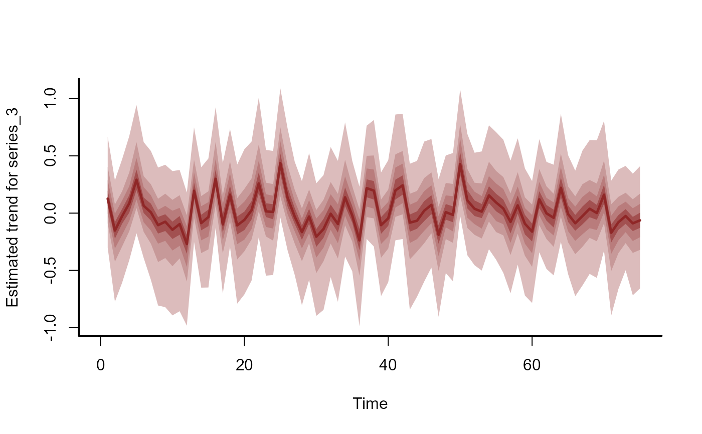
 plot(mod, type = "trend", series = 1)
 plot(mod, type = "trend", series = 2)
 plot(mod, type = "trend", series = 3)
 # =============================================================================
# Time-Varying (Dynamic) Coefficients
# =============================================================================
# Example of how to use dynamic coefficients
# Simulate a time-varying coefficient for the effect of temperature
set.seed(123)
N <- 200
beta_temp <- vector(length = N)
beta_temp[1] <- 0.4
for (i in 2:N) {
beta_temp[i] <- rnorm(1, mean = beta_temp[i - 1] - 0.0025, sd = 0.05)
}
plot(beta_temp)
# =============================================================================
# Time-Varying (Dynamic) Coefficients
# =============================================================================
# Example of how to use dynamic coefficients
# Simulate a time-varying coefficient for the effect of temperature
set.seed(123)
N <- 200
beta_temp <- vector(length = N)
beta_temp[1] <- 0.4
for (i in 2:N) {
beta_temp[i] <- rnorm(1, mean = beta_temp[i - 1] - 0.0025, sd = 0.05)
}
plot(beta_temp)
 # Simulate a covariate called 'temp'
temp <- rnorm(N, sd = 1)
# Simulate some noisy Gaussian observations
out <- rnorm(N,
mean = 4 + beta_temp * temp,
sd = 0.5
)
# Gather necessary data into a data.frame; split into training / testing
data <- data.frame(out, temp, time = seq_along(temp))
data_train <- data[1:180, ]
data_test <- data[181:200, ]
# Fit the model using the dynamic() function
mod <- mvgam(
formula = out ~ dynamic(
temp,
scale = FALSE,
k = 40
),
family = gaussian(),
data = data_train,
newdata = data_test,
chains = 2,
silent = 2
)
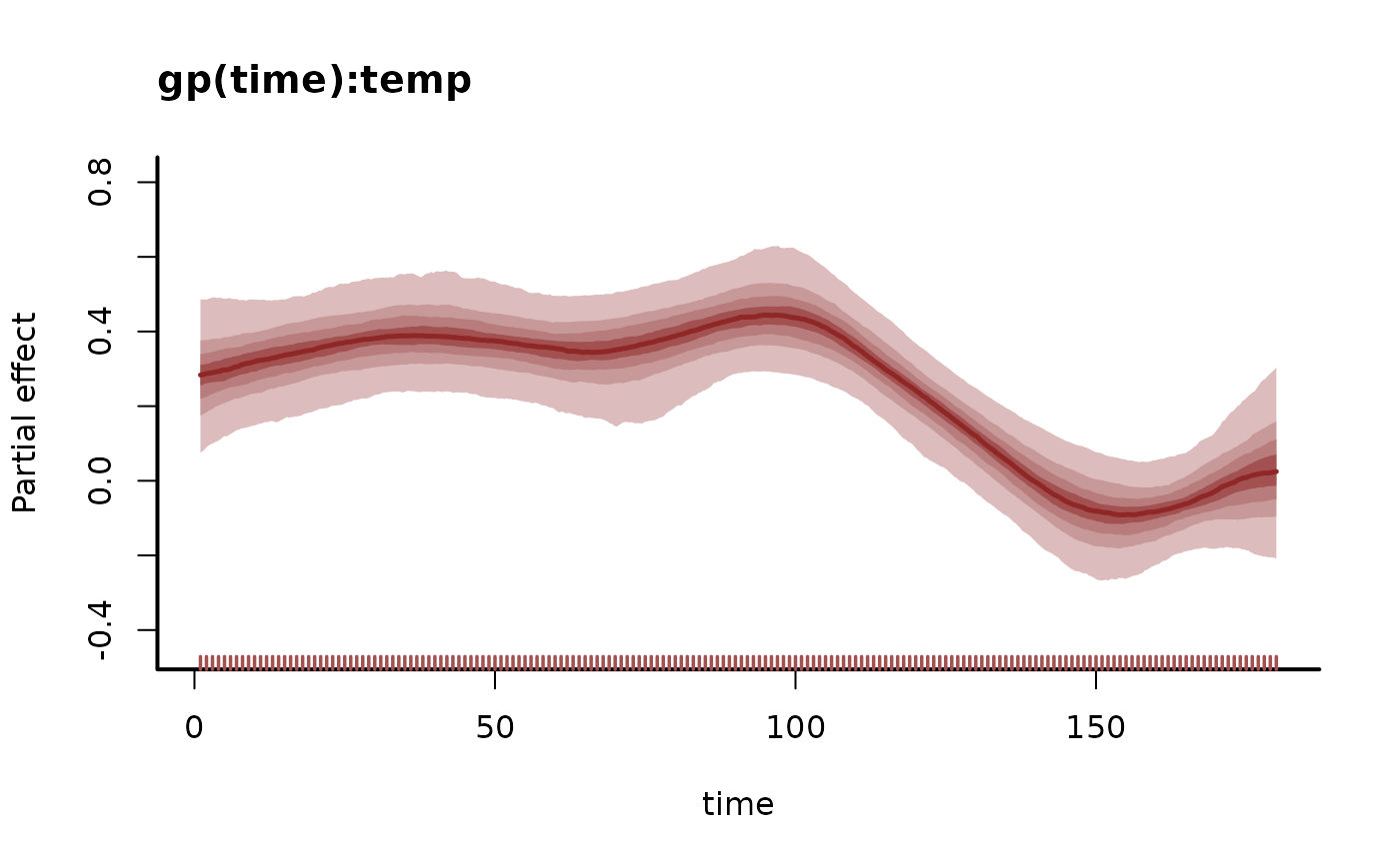
# Inspect the model summary, forecast and time-varying coefficient distribution
summary(mod)
#> GAM formula:
#> out ~ gp(time, by = temp, c = 5/4, k = 40, scale = FALSE)
#> <environment: 0x5582dd828d38>
#>
#> Family:
#> gaussian
#>
#> Link function:
#> identity
#>
#> Trend model:
#> None
#>
#> N series:
#> 1
#>
#> N timepoints:
#> 200
#>
#> Status:
#> Fitted using Stan
#> 2 chains, each with iter = 1000; warmup = 500; thin = 1
#> Total post-warmup draws = 1000
#>
#> Observation error parameter estimates:
#> 2.5% 50% 97.5% Rhat n_eff
#> sigma_obs[1] 0.44 0.49 0.54 1 1078
#>
#> GAM coefficient (beta) estimates:
#> 2.5% 50% 97.5% Rhat n_eff
#> (Intercept) 4.000 4.0e+00 4.1000 1.00 1167
#> gp(time):temp.1 1.000 3.3e+00 6.3000 1.00 710
#> gp(time):temp.2 -2.700 1.5e+00 5.8000 1.00 664
#> gp(time):temp.3 -5.500 -1.4e+00 3.1000 1.00 779
#> gp(time):temp.4 -5.300 -1.2e+00 2.6000 1.00 653
#> gp(time):temp.5 -3.000 4.3e-01 3.4000 1.00 869
#> gp(time):temp.6 -2.300 1.6e-01 3.3000 1.00 824
#> gp(time):temp.7 -3.400 -4.4e-01 1.9000 1.01 832
#> gp(time):temp.8 -1.600 2.4e-01 2.6000 1.00 883
#> gp(time):temp.9 -1.300 3.4e-01 2.8000 1.00 758
#> gp(time):temp.10 -2.500 -3.4e-01 0.9500 1.00 627
#> gp(time):temp.11 -1.700 -2.2e-02 1.2000 1.00 1218
#> gp(time):temp.12 -0.820 1.6e-01 1.9000 1.00 902
#> gp(time):temp.13 -1.200 -6.4e-14 1.3000 1.00 1070
#> gp(time):temp.14 -1.400 -3.1e-03 0.7800 1.00 1052
#> gp(time):temp.15 -0.810 1.0e-10 0.9800 1.00 1019
#> gp(time):temp.16 -0.790 1.4e-05 1.1000 1.00 1661
#> gp(time):temp.17 -0.810 1.3e-12 0.8300 1.00 1114
#> gp(time):temp.18 -0.630 1.5e-26 0.7000 1.00 1057
#> gp(time):temp.19 -0.930 -7.9e-06 0.2700 1.00 1059
#> gp(time):temp.20 -0.420 5.3e-17 0.4800 1.00 1253
#> gp(time):temp.21 -0.210 3.8e-10 0.7600 1.00 658
#> gp(time):temp.22 -0.400 -4.0e-16 0.2700 1.00 1133
#> gp(time):temp.23 -0.480 -3.1e-24 0.2700 1.00 883
#> gp(time):temp.24 -0.160 2.8e-17 0.6000 1.00 1074
#> gp(time):temp.25 -0.250 1.2e-20 0.2900 1.00 1258
#> gp(time):temp.26 -0.390 -5.6e-16 0.1600 1.00 692
#> gp(time):temp.27 -0.140 -1.6e-46 0.3100 1.00 1664
#> gp(time):temp.28 -0.100 1.4e-34 0.2500 1.00 562
#> gp(time):temp.29 -0.240 5.5e-59 0.1200 1.00 1525
#> gp(time):temp.30 -0.170 1.0e-84 0.1300 1.00 943
#> gp(time):temp.31 -0.097 -1.7e-41 0.1900 1.00 943
#> gp(time):temp.32 -0.075 3.2e-72 0.1300 1.00 1186
#> gp(time):temp.33 -0.110 3.6e-85 0.0700 1.00 1965
#> gp(time):temp.34 -0.041 6.7e-96 0.0870 1.01 401
#> gp(time):temp.35 -0.044 -1.3e-85 0.0610 1.00 1026
#> gp(time):temp.36 -0.042 6.9e-107 0.0350 1.00 883
#> gp(time):temp.37 -0.055 1.0e-74 0.0320 1.00 1548
#> gp(time):temp.38 -0.025 1.9e-62 0.0250 1.00 640
#> gp(time):temp.39 -0.018 -1.3e-69 0.0290 1.00 905
#> gp(time):temp.40 -0.031 -2.7e-64 0.0077 1.00 722
#>
#> GAM gp term marginal deviation (alpha) and length scale (rho) estimates:
#> 2.5% 50% 97.5% Rhat n_eff
#> alpha_gp(time):temp 0.18 0.34 0.88 1 242
#> rho_gp(time):temp 12.00 32.00 94.00 1 211
#>
#> Stan MCMC diagnostics:
#> ✔ No issues with effective samples per iteration
#> ✔ Rhat looks good for all parameters
#> ✔ No issues with divergences
#> ✔ No issues with maximum tree depth
#>
#> Samples were drawn using sampling(hmc). For each parameter, n_eff is a
#> crude measure of effective sample size, and Rhat is the potential scale
#> reduction factor on split MCMC chains (at convergence, Rhat = 1)
#>
#> Use how_to_cite() to get started describing this model
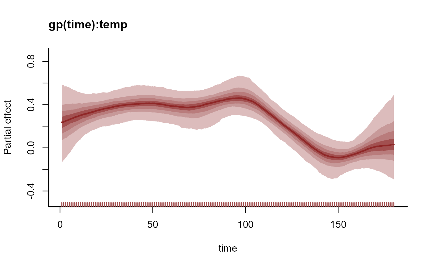
plot(mod, type = "smooths")
# Simulate a covariate called 'temp'
temp <- rnorm(N, sd = 1)
# Simulate some noisy Gaussian observations
out <- rnorm(N,
mean = 4 + beta_temp * temp,
sd = 0.5
)
# Gather necessary data into a data.frame; split into training / testing
data <- data.frame(out, temp, time = seq_along(temp))
data_train <- data[1:180, ]
data_test <- data[181:200, ]
# Fit the model using the dynamic() function
mod <- mvgam(
formula = out ~ dynamic(
temp,
scale = FALSE,
k = 40
),
family = gaussian(),
data = data_train,
newdata = data_test,
chains = 2,
silent = 2
)
# Inspect the model summary, forecast and time-varying coefficient distribution
summary(mod)
#> GAM formula:
#> out ~ gp(time, by = temp, c = 5/4, k = 40, scale = FALSE)
#> <environment: 0x5582dd828d38>
#>
#> Family:
#> gaussian
#>
#> Link function:
#> identity
#>
#> Trend model:
#> None
#>
#> N series:
#> 1
#>
#> N timepoints:
#> 200
#>
#> Status:
#> Fitted using Stan
#> 2 chains, each with iter = 1000; warmup = 500; thin = 1
#> Total post-warmup draws = 1000
#>
#> Observation error parameter estimates:
#> 2.5% 50% 97.5% Rhat n_eff
#> sigma_obs[1] 0.44 0.49 0.54 1 1078
#>
#> GAM coefficient (beta) estimates:
#> 2.5% 50% 97.5% Rhat n_eff
#> (Intercept) 4.000 4.0e+00 4.1000 1.00 1167
#> gp(time):temp.1 1.000 3.3e+00 6.3000 1.00 710
#> gp(time):temp.2 -2.700 1.5e+00 5.8000 1.00 664
#> gp(time):temp.3 -5.500 -1.4e+00 3.1000 1.00 779
#> gp(time):temp.4 -5.300 -1.2e+00 2.6000 1.00 653
#> gp(time):temp.5 -3.000 4.3e-01 3.4000 1.00 869
#> gp(time):temp.6 -2.300 1.6e-01 3.3000 1.00 824
#> gp(time):temp.7 -3.400 -4.4e-01 1.9000 1.01 832
#> gp(time):temp.8 -1.600 2.4e-01 2.6000 1.00 883
#> gp(time):temp.9 -1.300 3.4e-01 2.8000 1.00 758
#> gp(time):temp.10 -2.500 -3.4e-01 0.9500 1.00 627
#> gp(time):temp.11 -1.700 -2.2e-02 1.2000 1.00 1218
#> gp(time):temp.12 -0.820 1.6e-01 1.9000 1.00 902
#> gp(time):temp.13 -1.200 -6.4e-14 1.3000 1.00 1070
#> gp(time):temp.14 -1.400 -3.1e-03 0.7800 1.00 1052
#> gp(time):temp.15 -0.810 1.0e-10 0.9800 1.00 1019
#> gp(time):temp.16 -0.790 1.4e-05 1.1000 1.00 1661
#> gp(time):temp.17 -0.810 1.3e-12 0.8300 1.00 1114
#> gp(time):temp.18 -0.630 1.5e-26 0.7000 1.00 1057
#> gp(time):temp.19 -0.930 -7.9e-06 0.2700 1.00 1059
#> gp(time):temp.20 -0.420 5.3e-17 0.4800 1.00 1253
#> gp(time):temp.21 -0.210 3.8e-10 0.7600 1.00 658
#> gp(time):temp.22 -0.400 -4.0e-16 0.2700 1.00 1133
#> gp(time):temp.23 -0.480 -3.1e-24 0.2700 1.00 883
#> gp(time):temp.24 -0.160 2.8e-17 0.6000 1.00 1074
#> gp(time):temp.25 -0.250 1.2e-20 0.2900 1.00 1258
#> gp(time):temp.26 -0.390 -5.6e-16 0.1600 1.00 692
#> gp(time):temp.27 -0.140 -1.6e-46 0.3100 1.00 1664
#> gp(time):temp.28 -0.100 1.4e-34 0.2500 1.00 562
#> gp(time):temp.29 -0.240 5.5e-59 0.1200 1.00 1525
#> gp(time):temp.30 -0.170 1.0e-84 0.1300 1.00 943
#> gp(time):temp.31 -0.097 -1.7e-41 0.1900 1.00 943
#> gp(time):temp.32 -0.075 3.2e-72 0.1300 1.00 1186
#> gp(time):temp.33 -0.110 3.6e-85 0.0700 1.00 1965
#> gp(time):temp.34 -0.041 6.7e-96 0.0870 1.01 401
#> gp(time):temp.35 -0.044 -1.3e-85 0.0610 1.00 1026
#> gp(time):temp.36 -0.042 6.9e-107 0.0350 1.00 883
#> gp(time):temp.37 -0.055 1.0e-74 0.0320 1.00 1548
#> gp(time):temp.38 -0.025 1.9e-62 0.0250 1.00 640
#> gp(time):temp.39 -0.018 -1.3e-69 0.0290 1.00 905
#> gp(time):temp.40 -0.031 -2.7e-64 0.0077 1.00 722
#>
#> GAM gp term marginal deviation (alpha) and length scale (rho) estimates:
#> 2.5% 50% 97.5% Rhat n_eff
#> alpha_gp(time):temp 0.18 0.34 0.88 1 242
#> rho_gp(time):temp 12.00 32.00 94.00 1 211
#>
#> Stan MCMC diagnostics:
#> ✔ No issues with effective samples per iteration
#> ✔ Rhat looks good for all parameters
#> ✔ No issues with divergences
#> ✔ No issues with maximum tree depth
#>
#> Samples were drawn using sampling(hmc). For each parameter, n_eff is a
#> crude measure of effective sample size, and Rhat is the potential scale
#> reduction factor on split MCMC chains (at convergence, Rhat = 1)
#>
#> Use how_to_cite() to get started describing this model
plot(mod, type = "smooths")
 fc <- forecast(mod, newdata = data_test)
plot(fc)
#> Out of sample CRPS:
#> 6.35165092208796
fc <- forecast(mod, newdata = data_test)
plot(fc)
#> Out of sample CRPS:
#> 6.35165092208796
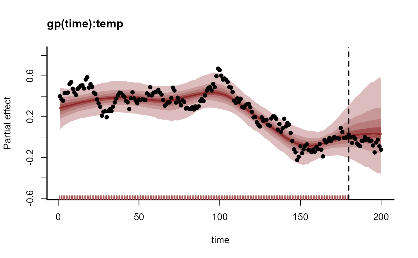
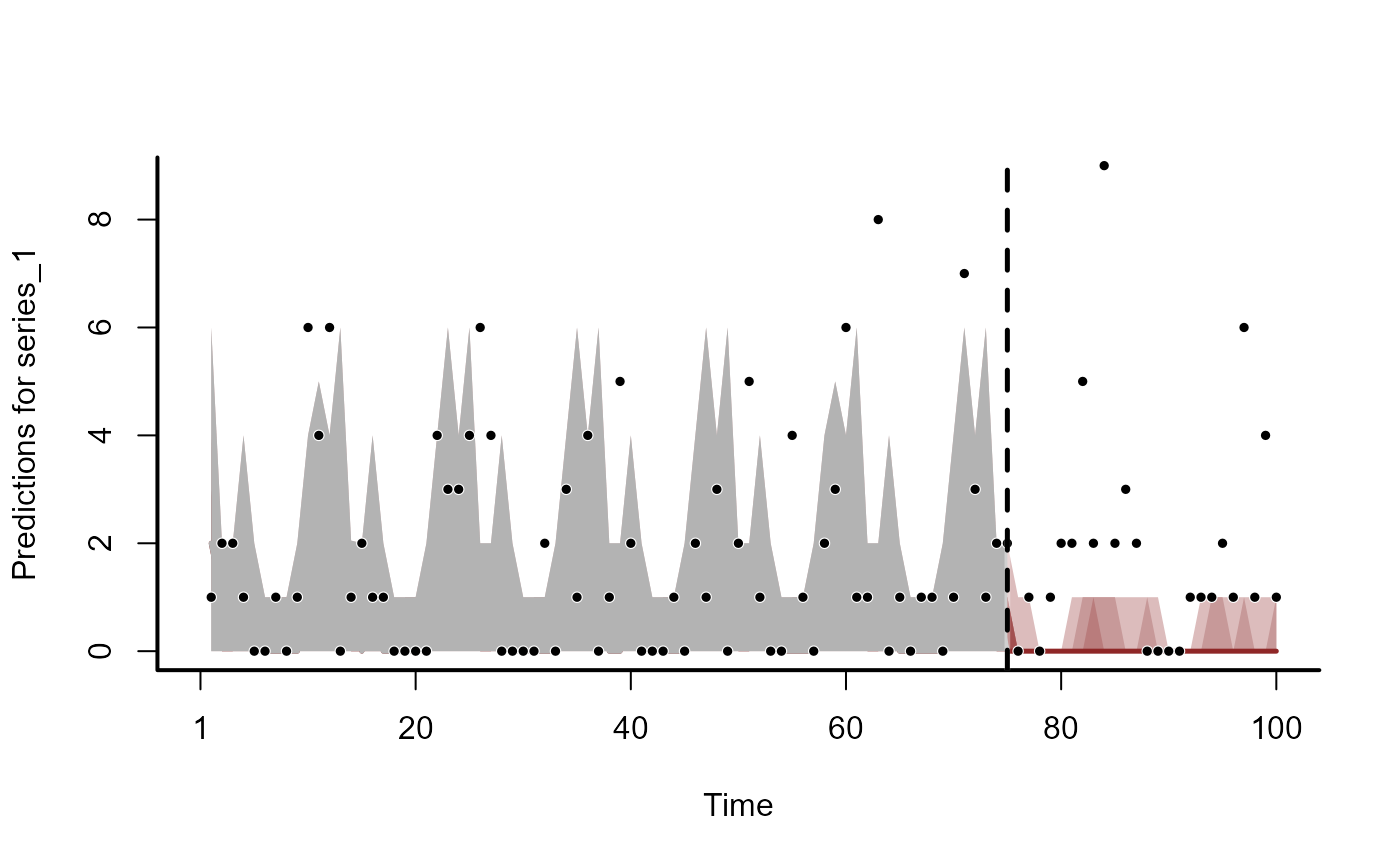
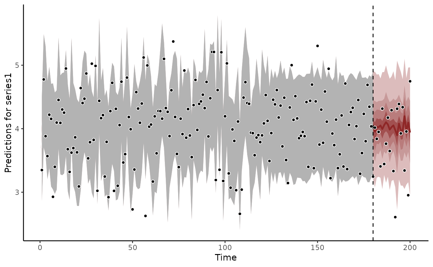 # Propagating the smooth term shows how the coefficient is expected to evolve
plot_mvgam_smooth(mod, smooth = 1, newdata = data)
abline(v = 180, lty = "dashed", lwd = 2)
points(beta_temp, pch = 16)
# Propagating the smooth term shows how the coefficient is expected to evolve
plot_mvgam_smooth(mod, smooth = 1, newdata = data)
abline(v = 180, lty = "dashed", lwd = 2)
points(beta_temp, pch = 16)
 # =============================================================================
# Working with Offset Terms
# =============================================================================
# Example showing how to incorporate an offset; simulate some count data
# with different means per series
set.seed(100)
dat <- sim_mvgam(
prop_trend = 0,
mu = c(0, 2, 2),
seasonality = "hierarchical"
)
# Add offset terms to the training and testing data
dat$data_train$offset <- 0.5 * as.numeric(dat$data_train$series)
dat$data_test$offset <- 0.5 * as.numeric(dat$data_test$series)
# Fit a model that includes the offset in the linear predictor as well as
# hierarchical seasonal smooths
mod <- mvgam(
formula = y ~ offset(offset) +
s(series, bs = "re") +
s(season, bs = "cc") +
s(season, by = series, m = 1, k = 5),
data = dat$data_train,
chains = 2,
silent = 2
)
# Inspect the model file to see the modification to the linear predictor (eta)
stancode(mod)
#> // Stan model code generated by package mvgam
#> data {
#> int<lower=0> total_obs; // total number of observations
#> int<lower=0> n; // number of timepoints per series
#> int<lower=0> n_sp; // number of smoothing parameters
#> int<lower=0> n_series; // number of series
#> int<lower=0> num_basis; // total number of basis coefficients
#> vector[num_basis] zero; // prior locations for basis coefficients
#> vector[total_obs] off_set; // offset vector
#> matrix[total_obs, num_basis] X; // mgcv GAM design matrix
#> array[n, n_series] int<lower=0> ytimes; // time-ordered matrix (which col in X belongs to each [time, series] observation?)
#> matrix[8, 8] S1; // mgcv smooth penalty matrix S1
#> matrix[4, 4] S2; // mgcv smooth penalty matrix S2
#> matrix[4, 4] S3; // mgcv smooth penalty matrix S3
#> matrix[4, 4] S4; // mgcv smooth penalty matrix S4
#> int<lower=0> n_nonmissing; // number of nonmissing observations
#> array[n_nonmissing] int<lower=0> flat_ys; // flattened nonmissing observations
#> matrix[n_nonmissing, num_basis] flat_xs; // X values for nonmissing observations
#> array[n_nonmissing] int<lower=0> obs_ind; // indices of nonmissing observations
#> }
#> parameters {
#> // raw basis coefficients
#> vector[num_basis] b_raw;
#>
#> // random effect variances
#> vector<lower=0>[1] sigma_raw;
#>
#> // random effect means
#> vector[1] mu_raw;
#>
#> // smoothing parameters
#> vector<lower=0>[n_sp] lambda;
#> }
#> transformed parameters {
#> // basis coefficients
#> vector[num_basis] b;
#> b[1 : 21] = b_raw[1 : 21];
#> b[22 : 24] = mu_raw[1] + b_raw[22 : 24] * sigma_raw[1];
#> }
#> model {
#> // prior for random effect population variances
#> sigma_raw ~ inv_gamma(1.418, 0.452);
#>
#> // prior for random effect population means
#> mu_raw ~ std_normal();
#>
#> // prior for (Intercept)...
#> b_raw[1] ~ student_t(3, 1.6, 2.5);
#>
#> // prior for s(season)...
#> b_raw[2 : 9] ~ multi_normal_prec(zero[2 : 9], S1[1 : 8, 1 : 8] * lambda[1]);
#>
#> // prior for s(season):seriesseries_1...
#> b_raw[10 : 13] ~ multi_normal_prec(zero[10 : 13],
#> S2[1 : 4, 1 : 4] * lambda[2]);
#>
#> // prior for s(season):seriesseries_2...
#> b_raw[14 : 17] ~ multi_normal_prec(zero[14 : 17],
#> S3[1 : 4, 1 : 4] * lambda[3]);
#>
#> // prior for s(season):seriesseries_3...
#> b_raw[18 : 21] ~ multi_normal_prec(zero[18 : 21],
#> S4[1 : 4, 1 : 4] * lambda[4]);
#>
#> // prior (non-centred) for s(series)...
#> b_raw[22 : 24] ~ std_normal();
#>
#> // priors for smoothing parameters
#> lambda ~ normal(5, 30);
#> {
#> // likelihood functions
#> flat_ys ~ poisson_log_glm(flat_xs, off_set[obs_ind], b);
#> }
#> }
#> generated quantities {
#> vector[total_obs] eta;
#> matrix[n, n_series] mus;
#> vector[n_sp] rho;
#> array[n, n_series] int ypred;
#> rho = log(lambda);
#>
#> // posterior predictions
#> eta = X * b + off_set;
#> for (s in 1 : n_series) {
#> mus[1 : n, s] = eta[ytimes[1 : n, s]];
#> ypred[1 : n, s] = poisson_log_rng(mus[1 : n, s]);
#> }
#> }
#>
#>
# Forecasts for the first two series will differ in magnitude
fc <- forecast(mod, newdata = dat$data_test)
plot(fc, series = 1, ylim = c(0, 75))
#> Out of sample DRPS:
#> 26.650371
# =============================================================================
# Working with Offset Terms
# =============================================================================
# Example showing how to incorporate an offset; simulate some count data
# with different means per series
set.seed(100)
dat <- sim_mvgam(
prop_trend = 0,
mu = c(0, 2, 2),
seasonality = "hierarchical"
)
# Add offset terms to the training and testing data
dat$data_train$offset <- 0.5 * as.numeric(dat$data_train$series)
dat$data_test$offset <- 0.5 * as.numeric(dat$data_test$series)
# Fit a model that includes the offset in the linear predictor as well as
# hierarchical seasonal smooths
mod <- mvgam(
formula = y ~ offset(offset) +
s(series, bs = "re") +
s(season, bs = "cc") +
s(season, by = series, m = 1, k = 5),
data = dat$data_train,
chains = 2,
silent = 2
)
# Inspect the model file to see the modification to the linear predictor (eta)
stancode(mod)
#> // Stan model code generated by package mvgam
#> data {
#> int<lower=0> total_obs; // total number of observations
#> int<lower=0> n; // number of timepoints per series
#> int<lower=0> n_sp; // number of smoothing parameters
#> int<lower=0> n_series; // number of series
#> int<lower=0> num_basis; // total number of basis coefficients
#> vector[num_basis] zero; // prior locations for basis coefficients
#> vector[total_obs] off_set; // offset vector
#> matrix[total_obs, num_basis] X; // mgcv GAM design matrix
#> array[n, n_series] int<lower=0> ytimes; // time-ordered matrix (which col in X belongs to each [time, series] observation?)
#> matrix[8, 8] S1; // mgcv smooth penalty matrix S1
#> matrix[4, 4] S2; // mgcv smooth penalty matrix S2
#> matrix[4, 4] S3; // mgcv smooth penalty matrix S3
#> matrix[4, 4] S4; // mgcv smooth penalty matrix S4
#> int<lower=0> n_nonmissing; // number of nonmissing observations
#> array[n_nonmissing] int<lower=0> flat_ys; // flattened nonmissing observations
#> matrix[n_nonmissing, num_basis] flat_xs; // X values for nonmissing observations
#> array[n_nonmissing] int<lower=0> obs_ind; // indices of nonmissing observations
#> }
#> parameters {
#> // raw basis coefficients
#> vector[num_basis] b_raw;
#>
#> // random effect variances
#> vector<lower=0>[1] sigma_raw;
#>
#> // random effect means
#> vector[1] mu_raw;
#>
#> // smoothing parameters
#> vector<lower=0>[n_sp] lambda;
#> }
#> transformed parameters {
#> // basis coefficients
#> vector[num_basis] b;
#> b[1 : 21] = b_raw[1 : 21];
#> b[22 : 24] = mu_raw[1] + b_raw[22 : 24] * sigma_raw[1];
#> }
#> model {
#> // prior for random effect population variances
#> sigma_raw ~ inv_gamma(1.418, 0.452);
#>
#> // prior for random effect population means
#> mu_raw ~ std_normal();
#>
#> // prior for (Intercept)...
#> b_raw[1] ~ student_t(3, 1.6, 2.5);
#>
#> // prior for s(season)...
#> b_raw[2 : 9] ~ multi_normal_prec(zero[2 : 9], S1[1 : 8, 1 : 8] * lambda[1]);
#>
#> // prior for s(season):seriesseries_1...
#> b_raw[10 : 13] ~ multi_normal_prec(zero[10 : 13],
#> S2[1 : 4, 1 : 4] * lambda[2]);
#>
#> // prior for s(season):seriesseries_2...
#> b_raw[14 : 17] ~ multi_normal_prec(zero[14 : 17],
#> S3[1 : 4, 1 : 4] * lambda[3]);
#>
#> // prior for s(season):seriesseries_3...
#> b_raw[18 : 21] ~ multi_normal_prec(zero[18 : 21],
#> S4[1 : 4, 1 : 4] * lambda[4]);
#>
#> // prior (non-centred) for s(series)...
#> b_raw[22 : 24] ~ std_normal();
#>
#> // priors for smoothing parameters
#> lambda ~ normal(5, 30);
#> {
#> // likelihood functions
#> flat_ys ~ poisson_log_glm(flat_xs, off_set[obs_ind], b);
#> }
#> }
#> generated quantities {
#> vector[total_obs] eta;
#> matrix[n, n_series] mus;
#> vector[n_sp] rho;
#> array[n, n_series] int ypred;
#> rho = log(lambda);
#>
#> // posterior predictions
#> eta = X * b + off_set;
#> for (s in 1 : n_series) {
#> mus[1 : n, s] = eta[ytimes[1 : n, s]];
#> ypred[1 : n, s] = poisson_log_rng(mus[1 : n, s]);
#> }
#> }
#>
#>
# Forecasts for the first two series will differ in magnitude
fc <- forecast(mod, newdata = dat$data_test)
plot(fc, series = 1, ylim = c(0, 75))
#> Out of sample DRPS:
#> 26.650371
 plot(fc, series = 2, ylim = c(0, 75))
#> Out of sample DRPS:
#> 101.645578
#> Warning: Removed 8 rows containing missing values or values outside the scale range
#> (`geom_ribbon()`).
#> Warning: Removed 6 rows containing missing values or values outside the scale range
#> (`geom_ribbon()`).
plot(fc, series = 2, ylim = c(0, 75))
#> Out of sample DRPS:
#> 101.645578
#> Warning: Removed 8 rows containing missing values or values outside the scale range
#> (`geom_ribbon()`).
#> Warning: Removed 6 rows containing missing values or values outside the scale range
#> (`geom_ribbon()`).
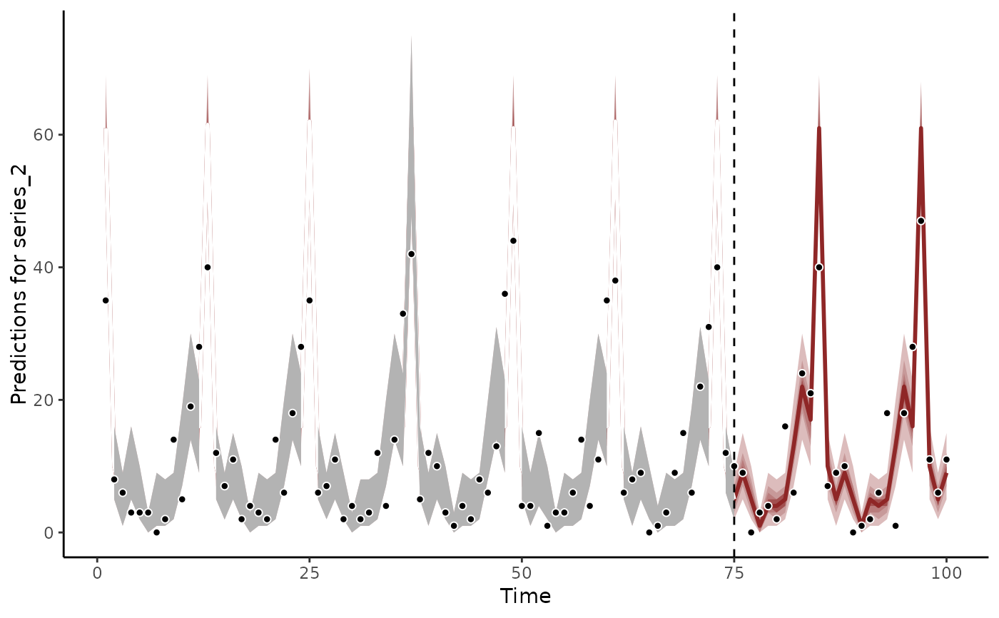 # Changing the offset for the testing data should lead to changes in
# the forecast
dat$data_test$offset <- dat$data_test$offset - 2
fc <- forecast(mod, newdata = dat$data_test)
plot(fc)
#> Out of sample DRPS:
#> 41.425863
# Changing the offset for the testing data should lead to changes in
# the forecast
dat$data_test$offset <- dat$data_test$offset - 2
fc <- forecast(mod, newdata = dat$data_test)
plot(fc)
#> Out of sample DRPS:
#> 41.425863
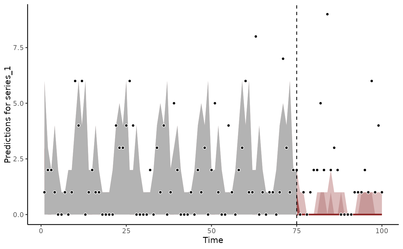 # Relative Risks can be computed by fixing the offset to the same value
# for each series
dat$data_test$offset <- rep(1, NROW(dat$data_test))
preds_rr <- predict(mod,
type = "link",
newdata = dat$data_test,
summary = FALSE
)
series1_inds <- which(dat$data_test$series == "series_1")
series2_inds <- which(dat$data_test$series == "series_2")
# Relative Risks are now more comparable among series
layout(matrix(1:2, ncol = 2))
plot(preds_rr[1, series1_inds],
type = "l", col = "grey75",
ylim = range(preds_rr),
ylab = "Series1 Relative Risk", xlab = "Time"
)
for (i in 2:50) {
lines(preds_rr[i, series1_inds], col = "grey75")
}
plot(preds_rr[1, series2_inds],
type = "l", col = "darkred",
ylim = range(preds_rr),
ylab = "Series2 Relative Risk", xlab = "Time"
)
for (i in 2:50) {
lines(preds_rr[i, series2_inds], col = "darkred")
}
# Relative Risks can be computed by fixing the offset to the same value
# for each series
dat$data_test$offset <- rep(1, NROW(dat$data_test))
preds_rr <- predict(mod,
type = "link",
newdata = dat$data_test,
summary = FALSE
)
series1_inds <- which(dat$data_test$series == "series_1")
series2_inds <- which(dat$data_test$series == "series_2")
# Relative Risks are now more comparable among series
layout(matrix(1:2, ncol = 2))
plot(preds_rr[1, series1_inds],
type = "l", col = "grey75",
ylim = range(preds_rr),
ylab = "Series1 Relative Risk", xlab = "Time"
)
for (i in 2:50) {
lines(preds_rr[i, series1_inds], col = "grey75")
}
plot(preds_rr[1, series2_inds],
type = "l", col = "darkred",
ylim = range(preds_rr),
ylab = "Series2 Relative Risk", xlab = "Time"
)
for (i in 2:50) {
lines(preds_rr[i, series2_inds], col = "darkred")
}
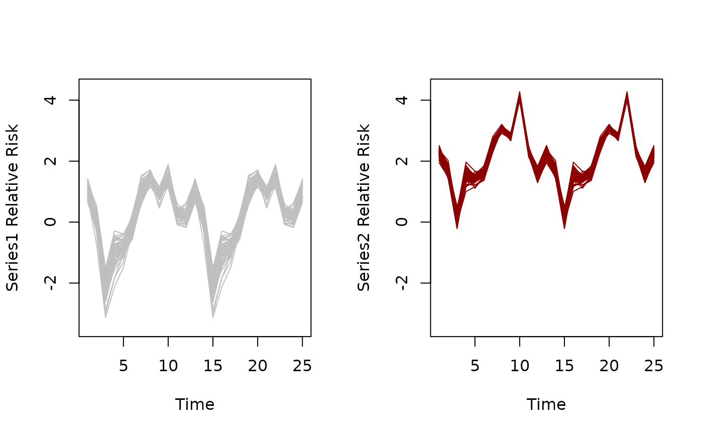 layout(1)
# =============================================================================
# Binomial Family Models
# =============================================================================
# Example showcasing how cbind() is needed for Binomial observations
# Simulate two time series of Binomial trials
trials <- sample(c(20:25), 50, replace = TRUE)
x <- rnorm(50)
detprob1 <- plogis(-0.5 + 0.9 * x)
detprob2 <- plogis(-0.1 - 0.7 * x)
dat <- rbind(
data.frame(
y = rbinom(n = 50, size = trials, prob = detprob1),
time = 1:50,
series = "series1",
x = x,
ntrials = trials
),
data.frame(
y = rbinom(n = 50, size = trials, prob = detprob2),
time = 1:50,
series = "series2",
x = x,
ntrials = trials
)
)
dat <- dplyr::mutate(dat, series = as.factor(series))
dat <- dplyr::arrange(dat, time, series)
plot_mvgam_series(data = dat, series = "all")
layout(1)
# =============================================================================
# Binomial Family Models
# =============================================================================
# Example showcasing how cbind() is needed for Binomial observations
# Simulate two time series of Binomial trials
trials <- sample(c(20:25), 50, replace = TRUE)
x <- rnorm(50)
detprob1 <- plogis(-0.5 + 0.9 * x)
detprob2 <- plogis(-0.1 - 0.7 * x)
dat <- rbind(
data.frame(
y = rbinom(n = 50, size = trials, prob = detprob1),
time = 1:50,
series = "series1",
x = x,
ntrials = trials
),
data.frame(
y = rbinom(n = 50, size = trials, prob = detprob2),
time = 1:50,
series = "series2",
x = x,
ntrials = trials
)
)
dat <- dplyr::mutate(dat, series = as.factor(series))
dat <- dplyr::arrange(dat, time, series)
plot_mvgam_series(data = dat, series = "all")
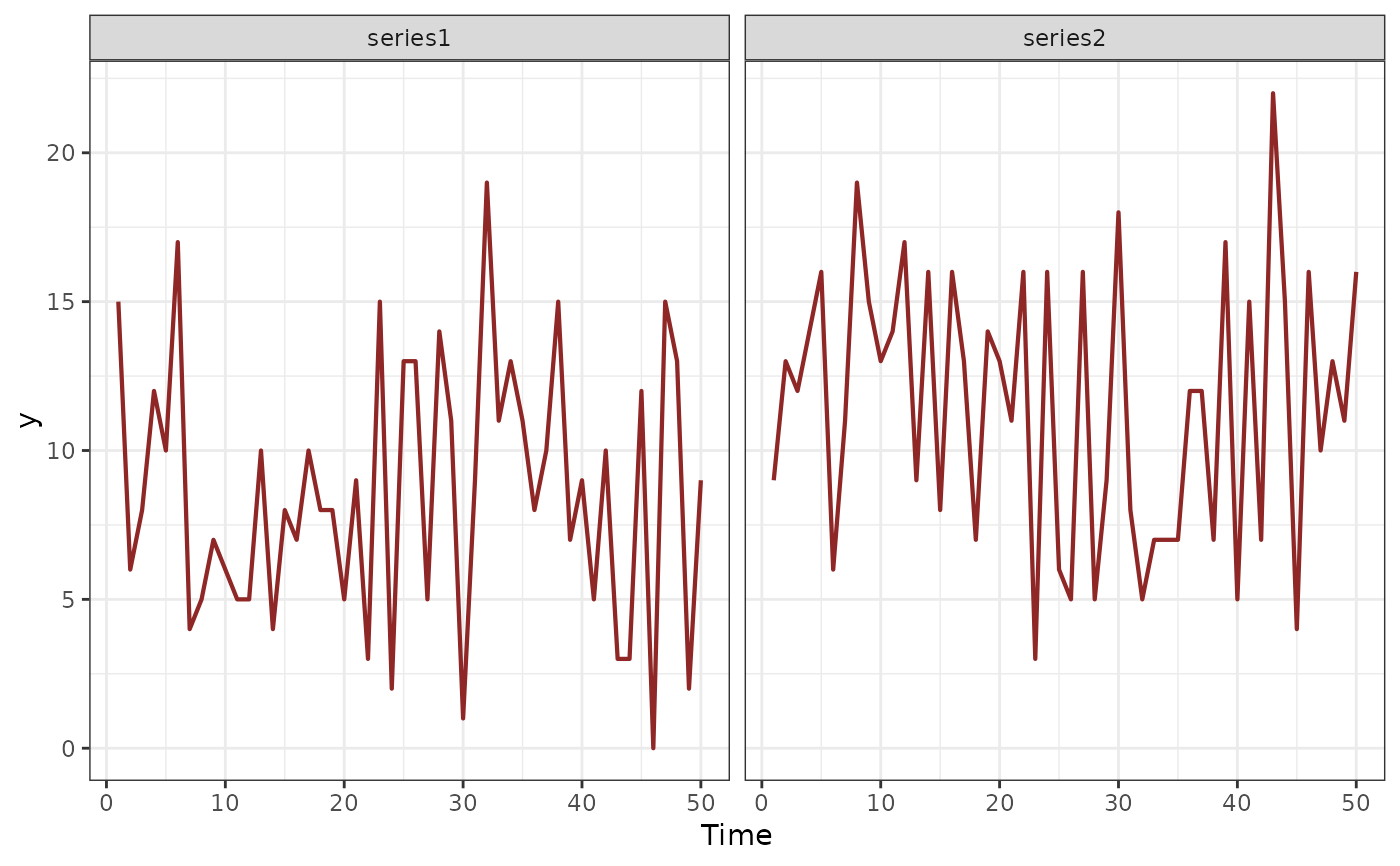 # Fit a model using the binomial() family; must specify observations
# and number of trials in the cbind() wrapper
mod <- mvgam(
formula = cbind(y, ntrials) ~ series + s(x, by = series),
family = binomial(),
data = dat,
chains = 2,
silent = 2
)
#> Warning: Binomial and Beta-binomial families require cbind(n_successes, n_trials)
#> in the formula left-hand side. Do not use cbind(n_successes, n_failures)!
#> This warning is displayed once per session.
summary(mod)
#> GAM formula:
#> cbind(y, ntrials) ~ series + s(x, by = series)
#> <environment: 0x5582dd828d38>
#>
#> Family:
#> binomial
#>
#> Link function:
#> logit
#>
#> Trend model:
#> None
#>
#> N series:
#> 2
#>
#> N timepoints:
#> 50
#>
#> Status:
#> Fitted using Stan
#> 2 chains, each with iter = 1000; warmup = 500; thin = 1
#> Total post-warmup draws = 1000
#>
#> GAM coefficient (beta) estimates:
#> 2.5% 50% 97.5% Rhat n_eff
#> (Intercept) -0.710 -0.5800 -0.440 1.00 610
#> seriesseries2 0.430 0.6000 0.790 1.00 601
#> s(x):seriesseries1.1 -0.680 -0.0780 0.110 1.03 55
#> s(x):seriesseries1.2 -0.520 -0.0130 0.450 1.01 245
#> s(x):seriesseries1.3 -0.260 -0.0180 0.037 1.02 80
#> s(x):seriesseries1.4 -0.260 -0.0094 0.230 1.01 256
#> s(x):seriesseries1.5 -0.040 0.0067 0.120 1.01 134
#> s(x):seriesseries1.6 -0.290 -0.0160 0.180 1.01 158
#> s(x):seriesseries1.7 -0.160 -0.0085 0.099 1.01 219
#> s(x):seriesseries1.8 -0.770 0.0510 0.990 1.01 238
#> s(x):seriesseries1.9 -0.033 0.6700 0.940 1.03 52
#> s(x):seriesseries2.1 -0.100 0.0470 0.640 1.01 61
#> s(x):seriesseries2.2 -0.160 0.0460 1.300 1.02 54
#> s(x):seriesseries2.3 -0.042 0.0110 0.250 1.02 49
#> s(x):seriesseries2.4 -0.100 0.0230 0.520 1.02 74
#> s(x):seriesseries2.5 -0.180 -0.0076 0.030 1.02 64
#> s(x):seriesseries2.6 -0.089 0.0250 0.570 1.02 61
#> s(x):seriesseries2.7 -0.046 0.0150 0.310 1.02 61
#> s(x):seriesseries2.8 -2.200 -0.1000 0.320 1.02 61
#> s(x):seriesseries2.9 -0.920 -0.6900 -0.110 1.01 70
#>
#> Approximate significance of GAM smooths:
#> edf Ref.df Chi.sq p-value
#> s(x):seriesseries1 4.204 9 59.27 0.000378 ***
#> s(x):seriesseries2 2.616 9 27.39 < 2e-16 ***
#> ---
#> Signif. codes: 0 ‘***’ 0.001 ‘**’ 0.01 ‘*’ 0.05 ‘.’ 0.1 ‘ ’ 1
#>
#> Stan MCMC diagnostics:
#> ✔ No issues with effective samples per iteration
#> ✔ Rhat looks good for all parameters
#> ✔ No issues with divergences
#> ✔ No issues with maximum tree depth
#>
#> Samples were drawn using sampling(hmc). For each parameter, n_eff is a
#> crude measure of effective sample size, and Rhat is the potential scale
#> reduction factor on split MCMC chains (at convergence, Rhat = 1)
#>
#> Use how_to_cite() to get started describing this model
pp_check(mod,
type = "bars_grouped",
group = "series", ndraws = 50
)
# Fit a model using the binomial() family; must specify observations
# and number of trials in the cbind() wrapper
mod <- mvgam(
formula = cbind(y, ntrials) ~ series + s(x, by = series),
family = binomial(),
data = dat,
chains = 2,
silent = 2
)
#> Warning: Binomial and Beta-binomial families require cbind(n_successes, n_trials)
#> in the formula left-hand side. Do not use cbind(n_successes, n_failures)!
#> This warning is displayed once per session.
summary(mod)
#> GAM formula:
#> cbind(y, ntrials) ~ series + s(x, by = series)
#> <environment: 0x5582dd828d38>
#>
#> Family:
#> binomial
#>
#> Link function:
#> logit
#>
#> Trend model:
#> None
#>
#> N series:
#> 2
#>
#> N timepoints:
#> 50
#>
#> Status:
#> Fitted using Stan
#> 2 chains, each with iter = 1000; warmup = 500; thin = 1
#> Total post-warmup draws = 1000
#>
#> GAM coefficient (beta) estimates:
#> 2.5% 50% 97.5% Rhat n_eff
#> (Intercept) -0.710 -0.5800 -0.440 1.00 610
#> seriesseries2 0.430 0.6000 0.790 1.00 601
#> s(x):seriesseries1.1 -0.680 -0.0780 0.110 1.03 55
#> s(x):seriesseries1.2 -0.520 -0.0130 0.450 1.01 245
#> s(x):seriesseries1.3 -0.260 -0.0180 0.037 1.02 80
#> s(x):seriesseries1.4 -0.260 -0.0094 0.230 1.01 256
#> s(x):seriesseries1.5 -0.040 0.0067 0.120 1.01 134
#> s(x):seriesseries1.6 -0.290 -0.0160 0.180 1.01 158
#> s(x):seriesseries1.7 -0.160 -0.0085 0.099 1.01 219
#> s(x):seriesseries1.8 -0.770 0.0510 0.990 1.01 238
#> s(x):seriesseries1.9 -0.033 0.6700 0.940 1.03 52
#> s(x):seriesseries2.1 -0.100 0.0470 0.640 1.01 61
#> s(x):seriesseries2.2 -0.160 0.0460 1.300 1.02 54
#> s(x):seriesseries2.3 -0.042 0.0110 0.250 1.02 49
#> s(x):seriesseries2.4 -0.100 0.0230 0.520 1.02 74
#> s(x):seriesseries2.5 -0.180 -0.0076 0.030 1.02 64
#> s(x):seriesseries2.6 -0.089 0.0250 0.570 1.02 61
#> s(x):seriesseries2.7 -0.046 0.0150 0.310 1.02 61
#> s(x):seriesseries2.8 -2.200 -0.1000 0.320 1.02 61
#> s(x):seriesseries2.9 -0.920 -0.6900 -0.110 1.01 70
#>
#> Approximate significance of GAM smooths:
#> edf Ref.df Chi.sq p-value
#> s(x):seriesseries1 4.204 9 59.27 0.000378 ***
#> s(x):seriesseries2 2.616 9 27.39 < 2e-16 ***
#> ---
#> Signif. codes: 0 ‘***’ 0.001 ‘**’ 0.01 ‘*’ 0.05 ‘.’ 0.1 ‘ ’ 1
#>
#> Stan MCMC diagnostics:
#> ✔ No issues with effective samples per iteration
#> ✔ Rhat looks good for all parameters
#> ✔ No issues with divergences
#> ✔ No issues with maximum tree depth
#>
#> Samples were drawn using sampling(hmc). For each parameter, n_eff is a
#> crude measure of effective sample size, and Rhat is the potential scale
#> reduction factor on split MCMC chains (at convergence, Rhat = 1)
#>
#> Use how_to_cite() to get started describing this model
pp_check(mod,
type = "bars_grouped",
group = "series", ndraws = 50
)
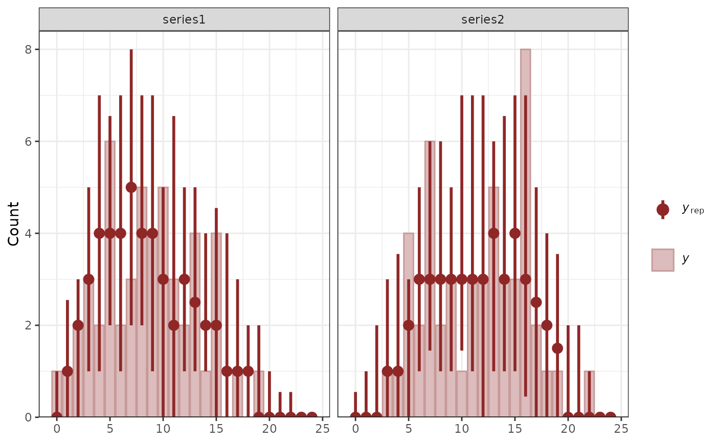 pp_check(mod,
type = "ecdf_overlay_grouped",
group = "series", ndraws = 50
)
pp_check(mod,
type = "ecdf_overlay_grouped",
group = "series", ndraws = 50
)
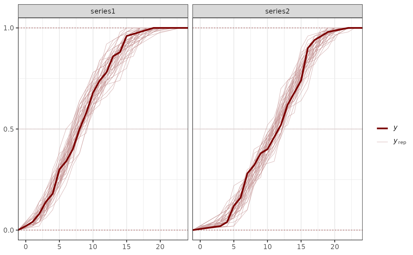 conditional_effects(mod, type = "link")
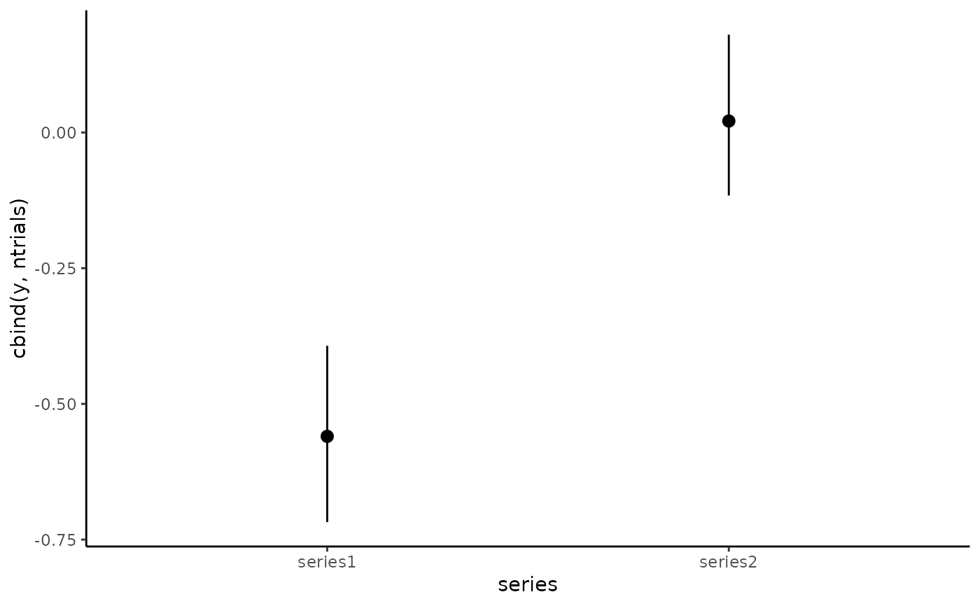
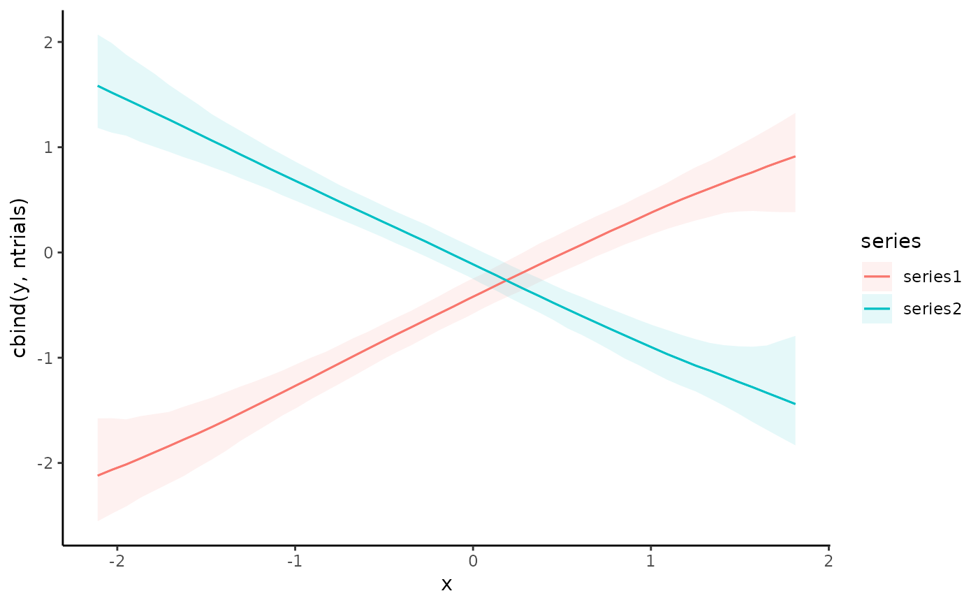 # To view predictions on the probability scale,
# use ntrials = 1 in datagrid()
plot_predictions(
mod,
by = c('x', 'series'),
newdata = datagrid(
x = runif(100, -2, 2),
series = unique,
ntrials = 1
),
type = 'expected'
)
# To view predictions on the probability scale,
# use ntrials = 1 in datagrid()
plot_predictions(
mod,
by = c('x', 'series'),
newdata = datagrid(
x = runif(100, -2, 2),
series = unique,
ntrials = 1
),
type = 'expected'
)
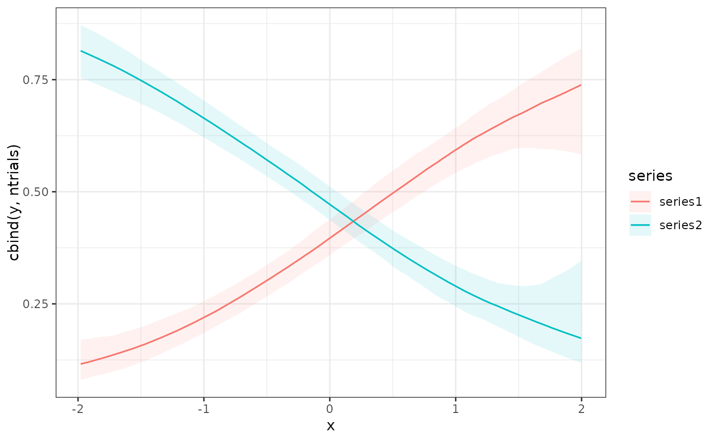 # Not needed for general use; cleans up connections for automated testing
closeAllConnections()
# }
# Not needed for general use; cleans up connections for automated testing
closeAllConnections()
# }