Shared latent states in mvgam

This vignette gives an example of how mvgam can be used to estimate models where multiple observed time series share the same latent process model. For full details on the basic mvgam functionality, please see the introductory vignette.

The `trend_map` argument

The trend_map argument in the mvgam() function is an optional data.frame that can be used to specify which series should depend on which latent process models (called “trends” in mvgam). This can be particularly useful if we wish to force multiple observed time series to depend on the same latent trend process, but with different observation processes. If this argument is supplied, a latent factor model is set up by setting use_lv = TRUE and using the supplied trend_map to set up the shared trends. Users familiar with the MARSS family of packages will recognize this as a way of specifying the \(Z\) matrix. This data.frame needs to have column names series and trend, with integer values in the trend column to state which trend each series should depend on. The series column should have a single unique entry for each time series in the data, with names that perfectly match the factor levels of the series variable in data). For example, if we were to simulate a collection of three integer-valued time series (using sim_mvgam), the following trend_map would force the first two series to share the same latent trend process:

set.seed(122)
simdat <- sim_mvgam(trend_model = 'AR1',
                    prop_trend = 0.6,
                    mu = c(0, 1, 2),
                    family = poisson())
trend_map <- data.frame(series = unique(simdat$data_train$series),
                        trend = c(1, 1, 2))
trend_map

##     series trend
## 1 series_1     1
## 2 series_2     1
## 3 series_3     2

We can see that the factor levels in trend_map match those in the data:

all.equal(levels(trend_map$series), levels(simdat$data_train$series))

## [1] TRUE

Checking `trend_map` with `run_model = FALSE`

Supplying this trend_map to the mvgam function for a simple model, but setting run_model = FALSE, allows us to inspect the constructed Stan code and the data objects that would be used to condition the model. Here we will set up a model in which each series has a different observation process (with only a different intercept per series in this case), and the two latent dynamic process models evolve as independent AR1 processes that also contain a shared nonlinear smooth function to capture repeated seasonality. This model is not too complicated but it does show how we can learn shared and independent effects for collections of time series in the mvgam framework:

fake_mod <- mvgam(y ~ 
                    # observation model formula, which has a 
                    # different intercept per series
                    series - 1,
                  
                  # process model formula, which has a shared seasonal smooth
                  # (each latent process model shares the SAME smooth)
                  trend_formula = ~ s(season, bs = 'cc', k = 6),
                  
                  # AR1 dynamics (each latent process model has DIFFERENT)
                  # dynamics
                  trend_model = 'AR1',
                  
                  # supplied trend_map
                  trend_map = trend_map,
                  
                  # data and observation family
                  family = poisson(),
                  data = simdat$data_train,
                  run_model = FALSE)

Inspecting the Stan code shows how this model is a dynamic factor model in which the loadings are constructed to reflect the supplied trend_map:

code(fake_mod)

## // Stan model code generated by package mvgam
## data {
##   int<lower=0> total_obs; // total number of observations
##   int<lower=0> n; // number of timepoints per series
##   int<lower=0> n_sp_trend; // number of trend smoothing parameters
##   int<lower=0> n_lv; // number of dynamic factors
##   int<lower=0> n_series; // number of series
##   matrix[n_series, n_lv] Z; // matrix mapping series to latent states
##   int<lower=0> num_basis; // total number of basis coefficients
##   int<lower=0> num_basis_trend; // number of trend basis coefficients
##   vector[num_basis_trend] zero_trend; // prior locations for trend basis coefficients
##   matrix[total_obs, num_basis] X; // mgcv GAM design matrix
##   matrix[n * n_lv, num_basis_trend] X_trend; // trend model design matrix
##   array[n, n_series] int<lower=0> ytimes; // time-ordered matrix (which col in X belongs to each [time, series] observation?)
##   array[n, n_lv] int ytimes_trend;
##   int<lower=0> n_nonmissing; // number of nonmissing observations
##   matrix[4, 4] S_trend1; // mgcv smooth penalty matrix S_trend1
##   array[n_nonmissing] int<lower=0> flat_ys; // flattened nonmissing observations
##   matrix[n_nonmissing, num_basis] flat_xs; // X values for nonmissing observations
##   array[n_nonmissing] int<lower=0> obs_ind; // indices of nonmissing observations
## }
## transformed data {
##   
## }
## parameters {
##   // raw basis coefficients
##   vector[num_basis] b_raw;
##   vector[num_basis_trend] b_raw_trend;
##   
##   // latent state SD terms
##   vector<lower=0>[n_lv] sigma;
##   
##   // latent state AR1 terms
##   vector<lower=-1.5, upper=1.5>[n_lv] ar1;
##   
##   // latent states
##   matrix[n, n_lv] LV;
##   
##   // smoothing parameters
##   vector<lower=0>[n_sp_trend] lambda_trend;
## }
## transformed parameters {
##   // latent states and loading matrix
##   vector[n * n_lv] trend_mus;
##   matrix[n, n_series] trend;
##   
##   // basis coefficients
##   vector[num_basis] b;
##   vector[num_basis_trend] b_trend;
##   
##   // observation model basis coefficients
##   b[1 : num_basis] = b_raw[1 : num_basis];
##   
##   // process model basis coefficients
##   b_trend[1 : num_basis_trend] = b_raw_trend[1 : num_basis_trend];
##   
##   // latent process linear predictors
##   trend_mus = X_trend * b_trend;
##   
##   // derived latent states
##   for (i in 1 : n) {
##     for (s in 1 : n_series) {
##       trend[i, s] = dot_product(Z[s,  : ], LV[i,  : ]);
##     }
##   }
## }
## model {
##   // prior for seriesseries_1...
##   b_raw[1] ~ student_t(3, 0, 2);
##   
##   // prior for seriesseries_2...
##   b_raw[2] ~ student_t(3, 0, 2);
##   
##   // prior for seriesseries_3...
##   b_raw[3] ~ student_t(3, 0, 2);
##   
##   // priors for AR parameters
##   ar1 ~ std_normal();
##   
##   // priors for latent state SD parameters
##   sigma ~ student_t(3, 0, 2.5);
##   
##   // dynamic process models
##   
##   // prior for s(season)_trend...
##   b_raw_trend[1 : 4] ~ multi_normal_prec(zero_trend[1 : 4],
##                                          S_trend1[1 : 4, 1 : 4]
##                                          * lambda_trend[1]);
##   lambda_trend ~ normal(5, 30);
##   for (j in 1 : n_lv) {
##     LV[1, j] ~ normal(trend_mus[ytimes_trend[1, j]], sigma[j]);
##     for (i in 2 : n) {
##       LV[i, j] ~ normal(trend_mus[ytimes_trend[i, j]]
##                         + ar1[j]
##                           * (LV[i - 1, j] - trend_mus[ytimes_trend[i - 1, j]]),
##                         sigma[j]);
##     }
##   }
##   {
##     // likelihood functions
##     vector[n_nonmissing] flat_trends;
##     flat_trends = to_vector(trend)[obs_ind];
##     flat_ys ~ poisson_log_glm(append_col(flat_xs, flat_trends), 0.0,
##                               append_row(b, 1.0));
##   }
## }
## generated quantities {
##   vector[total_obs] eta;
##   matrix[n, n_series] mus;
##   vector[n_sp_trend] rho_trend;
##   vector[n_lv] penalty;
##   array[n, n_series] int ypred;
##   penalty = 1.0 / (sigma .* sigma);
##   rho_trend = log(lambda_trend);
##   
##   matrix[n_series, n_lv] lv_coefs = Z;
##   // posterior predictions
##   eta = X * b;
##   for (s in 1 : n_series) {
##     mus[1 : n, s] = eta[ytimes[1 : n, s]] + trend[1 : n, s];
##     ypred[1 : n, s] = poisson_log_rng(mus[1 : n, s]);
##   }
## }

Notice the line that states “lv_coefs = Z;”. This uses the supplied \(Z\) matrix to construct the loading coefficients. The supplied matrix now looks exactly like what you’d use if you were to create a similar model in the MARSS package:

fake_mod$model_data$Z

##      [,1] [,2]
## [1,]    1    0
## [2,]    1    0
## [3,]    0    1

Fitting and inspecting the model

Though this model doesn’t perfectly match the data-generating process (which allowed each series to have different underlying dynamics), we can still fit it to show what the resulting inferences look like:

full_mod <- mvgam(y ~ series - 1,
                  trend_formula = ~ s(season, bs = 'cc', k = 6),
                  trend_model = 'AR1',
                  trend_map = trend_map,
                  family = poisson(),
                  data = simdat$data_train)

The summary of this model is informative as it shows that only two latent process models have been estimated, even though we have three observed time series. The model converges well

summary(full_mod)

## GAM observation formula:
## y ~ series - 1
## 
## GAM process formula:
## ~s(season, bs = "cc", k = 6)
## 
## Family:
## poisson
## 
## Link function:
## log
## 
## Trend model:
## AR1
## 
## N process models:
## 2 
## 
## N series:
## 3 
## 
## N timepoints:
## 75 
## 
## Status:
## Fitted using Stan 
## 4 chains, each with iter = 1000; warmup = 500; thin = 1 
## Total post-warmup draws = 2000
## 
## 
## GAM observation model coefficient (beta) estimates:
##                 2.5%   50% 97.5% Rhat n_eff
## seriesseries_1 -0.15 0.088  0.31 1.00  1895
## seriesseries_2  0.92 1.100  1.20 1.00  1267
## seriesseries_3  1.90 2.100  2.30 1.02   256
## 
## Process model AR parameter estimates:
##         2.5%    50%  97.5% Rhat n_eff
## ar1[1] -0.72 -0.420 -0.056    1   676
## ar1[2] -0.28 -0.011  0.280    1  1433
## 
## Process error parameter estimates:
##          2.5%  50% 97.5% Rhat n_eff
## sigma[1] 0.33 0.49  0.67    1   487
## sigma[2] 0.59 0.73  0.91    1   948
## 
## GAM process model coefficient (beta) estimates:
##                    2.5%    50% 97.5% Rhat n_eff
## s(season).1_trend -0.22 -0.011  0.20    1  1612
## s(season).2_trend -0.27 -0.045  0.18    1  1745
## s(season).3_trend -0.15  0.074  0.29    1  1347
## s(season).4_trend -0.15  0.067  0.28    1  1561
## 
## Approximate significance of GAM process smooths:
##            edf Ref.df    F p-value
## s(season) 1.52      4 0.21    0.92
## 
## Stan MCMC diagnostics:
## n_eff / iter looks reasonable for all parameters
## Rhat looks reasonable for all parameters
## 0 of 2000 iterations ended with a divergence (0%)
## 0 of 2000 iterations saturated the maximum tree depth of 12 (0%)
## E-FMI indicated no pathological behavior
## 
## Samples were drawn using NUTS(diag_e) at Mon Mar 25 1:53:19 PM 2024.
## For each parameter, n_eff is a crude measure of effective sample size,
## and Rhat is the potential scale reduction factor on split MCMC chains
## (at convergence, Rhat = 1)

Quick plots of all main effects can be made using conditional_effects():

plot(conditional_effects(full_mod, type = 'link'), ask = FALSE)

Even more informative are the plots of the latent processes. Both series 1 and 2 share the exact same estimates, while the estimates for series 3 are different:

plot(full_mod, type = 'trend', series = 1)

plot(full_mod, type = 'trend', series = 2)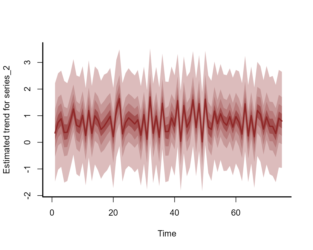

plot(full_mod, type = 'trend', series = 3)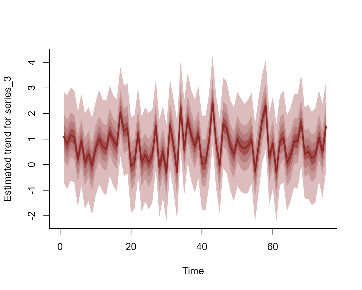

However, the forecasts for series’ 1 and 2 differ because they have different intercepts in the observation model

plot(full_mod, type = 'forecast', series = 1)

plot(full_mod, type = 'forecast', series = 2)

plot(full_mod, type = 'forecast', series = 3)

Example: signal detection

Now we will explore a more complicated example. Here we simulate a true hidden signal that we are trying to track. This signal depends nonlinearly on some covariate (called productivity, which represents a measure of how productive the landscape is). The signal also demonstrates a fairly large amount of temporal autocorrelation:

set.seed(543210)
# simulate a nonlinear relationship using the mgcv function gamSim
signal_dat <- gamSim(n = 100, eg = 1, scale = 1)

## Gu & Wahba 4 term additive model

# productivity is one of the variables in the simulated data
productivity <- signal_dat$x2

# simulate the true signal, which already has a nonlinear relationship
# with productivity; we will add in a fairly strong AR1 process to 
# contribute to the signal
true_signal <- as.vector(scale(signal_dat$y) +
                         arima.sim(100, model = list(ar = 0.8, sd = 0.1)))

Plot the signal to inspect it’s evolution over time

plot(true_signal, type = 'l',
     bty = 'l', lwd = 2,
     ylab = 'True signal',
     xlab = 'Time')

And plot the relationship between the signal and the productivity covariate:

plot(true_signal ~ productivity,
     pch = 16, bty = 'l',
     ylab = 'True signal',
     xlab = 'Productivity')

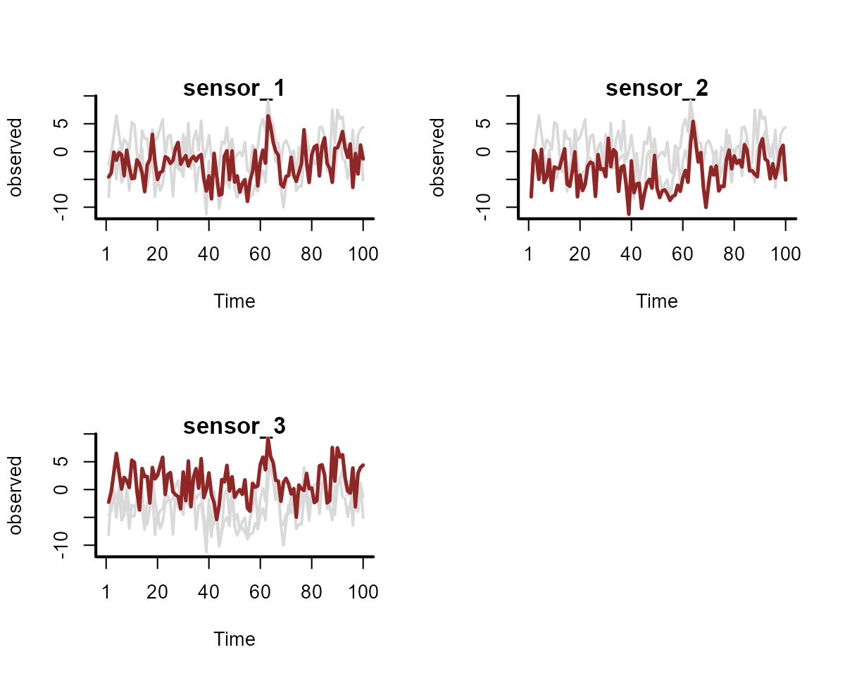
Next we simulate three sensors that are trying to track the same hidden signal. All of these sensors have different observation errors that can depend nonlinearly on a second external covariate, called temperature in this example. Again this makes use of gamSim

set.seed(543210)
sim_series = function(n_series = 3, true_signal){
  temp_effects <- gamSim(n = 100, eg = 7, scale = 0.1)
  temperature <- temp_effects$y
  alphas <- rnorm(n_series, sd = 2)

  do.call(rbind, lapply(seq_len(n_series), function(series){
    data.frame(observed = rnorm(length(true_signal),
                                mean = alphas[series] +
                                       1.5*as.vector(scale(temp_effects[, series + 1])) +
                                       true_signal,
                                sd = runif(1, 1, 2)),
               series = paste0('sensor_', series),
               time = 1:length(true_signal),
               temperature = temperature,
               productivity = productivity,
               true_signal = true_signal)
   }))
  }
model_dat <- sim_series(true_signal = true_signal) %>%
  dplyr::mutate(series = factor(series))

## Gu & Wahba 4 term additive model, correlated predictors

Plot the sensor observations

plot_mvgam_series(data = model_dat, y = 'observed',
                  series = 'all')

And now plot the observed relationships between the three sensors and the temperature covariate

 plot(observed ~ temperature, data = model_dat %>%
   dplyr::filter(series == 'sensor_1'),
   pch = 16, bty = 'l',
   ylab = 'Sensor 1',
   xlab = 'Temperature')

 plot(observed ~ temperature, data = model_dat %>%
   dplyr::filter(series == 'sensor_2'),
   pch = 16, bty = 'l',
   ylab = 'Sensor 2',
   xlab = 'Temperature')

 plot(observed ~ temperature, data = model_dat %>%
   dplyr::filter(series == 'sensor_3'),
   pch = 16, bty = 'l',
   ylab = 'Sensor 3',
   xlab = 'Temperature')

The shared signal model

Now we can formulate and fit a model that allows each sensor’s observation error to depend nonlinearly on temperature while allowing the true signal to depend nonlinearly on productivity. By fixing all of the values in the trend column to 1 in the trend_map, we are assuming that all observation sensors are tracking the same latent signal. We use informative priors on the two variance components (process error and observation error), which reflect our prior belief that the observation error is smaller overall than the true process error

mod <- mvgam(formula =
               # formula for observations, allowing for different
               # intercepts and hierarchical smooth effects of temperature
               observed ~ series + 
               s(temperature, k = 10) +
               s(series, temperature, bs = 'sz', k = 8),
             
             trend_formula =
               # formula for the latent signal, which can depend
               # nonlinearly on productivity
               ~ s(productivity, k = 8),
             
             trend_model =
               # in addition to productivity effects, the signal is
               # assumed to exhibit temporal autocorrelation
               'AR1',
             
             trend_map =
               # trend_map forces all sensors to track the same
               # latent signal
               data.frame(series = unique(model_dat$series),
                          trend = c(1, 1, 1)),
             
             # informative priors on process error
             # and observation error will help with convergence
             priors = c(prior(normal(2, 0.5), class = sigma),
                        prior(normal(1, 0.5), class = sigma_obs)),
             
             # Gaussian observations
             family = gaussian(),
             data = model_dat)

View a reduced version of the model summary because there will be many spline coefficients in this model

summary(mod, include_betas = FALSE)

## GAM observation formula:
## observed ~ series + s(temperature, k = 10) + s(series, temperature, 
##     bs = "sz", k = 8)
## 
## GAM process formula:
## ~s(productivity, k = 8)
## 
## Family:
## gaussian
## 
## Link function:
## identity
## 
## Trend model:
## AR1
## 
## N process models:
## 1 
## 
## N series:
## 3 
## 
## N timepoints:
## 100 
## 
## Status:
## Fitted using Stan 
## 4 chains, each with iter = 1100; warmup = 600; thin = 1 
## Total post-warmup draws = 2000
## 
## 
## Observation error parameter estimates:
##              2.5% 50% 97.5% Rhat n_eff
## sigma_obs[1]  1.6 1.9   2.2    1  1757
## sigma_obs[2]  1.4 1.7   2.0    1  1090
## sigma_obs[3]  1.3 1.5   1.8    1  1339
## 
## GAM observation model coefficient (beta) estimates:
##                 2.5%   50% 97.5% Rhat n_eff
## (Intercept)     0.72  1.70  2.50 1.01   360
## seriessensor_2 -2.10 -0.96  0.32 1.00  1068
## seriessensor_3 -3.40 -2.00 -0.39 1.00  1154
## 
## Approximate significance of GAM observation smooths:
##                        edf Ref.df    F p-value    
## s(temperature)        1.22      9 12.7  <2e-16 ***
## s(series,temperature) 1.92     16  1.0   0.011 *  
## ---
## Signif. codes:  0 '***' 0.001 '**' 0.01 '*' 0.05 '.' 0.1 ' ' 1
## 
## Process model AR parameter estimates:
##        2.5%  50% 97.5% Rhat n_eff
## ar1[1] 0.33 0.59  0.83    1   492
## 
## Process error parameter estimates:
##          2.5% 50% 97.5% Rhat n_eff
## sigma[1] 0.72   1   1.3 1.01   392
## 
## Approximate significance of GAM process smooths:
##                 edf Ref.df    F p-value    
## s(productivity) 3.6      7 9.34 0.00036 ***
## ---
## Signif. codes:  0 '***' 0.001 '**' 0.01 '*' 0.05 '.' 0.1 ' ' 1
## 
## Stan MCMC diagnostics:
## n_eff / iter looks reasonable for all parameters
## Rhats above 1.05 found for 28 parameters
##  *Diagnose further to investigate why the chains have not mixed
## 0 of 2000 iterations ended with a divergence (0%)
## 0 of 2000 iterations saturated the maximum tree depth of 12 (0%)
## E-FMI indicated no pathological behavior
## 
## Samples were drawn using NUTS(diag_e) at Mon Mar 25 1:55:37 PM 2024.
## For each parameter, n_eff is a crude measure of effective sample size,
## and Rhat is the potential scale reduction factor on split MCMC chains
## (at convergence, Rhat = 1)

Inspecting effects on both process and observation models

Don’t pay much attention to the approximate p-values of the smooth terms. The calculation for these values is incredibly sensitive to the estimates for the smoothing parameters so I don’t tend to find them to be very meaningful. What are meaningful, however, are prediction-based plots of the smooth functions. For example, here is the estimated response of the underlying signal to productivity:

plot(mod, type = 'smooths', trend_effects = TRUE)

And here are the estimated relationships between the sensor observations and the temperature covariate:

plot(mod, type = 'smooths')

All main effects can be quickly plotted with conditional_effects:

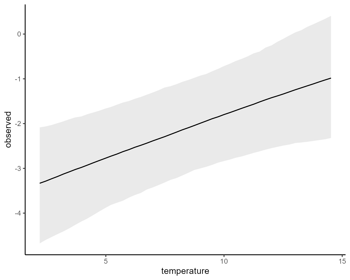
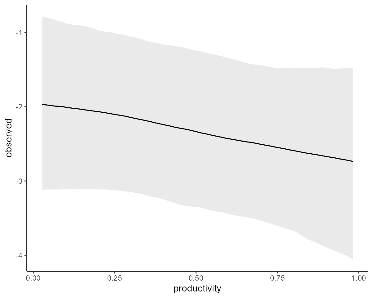
plot(conditional_effects(mod, type = 'link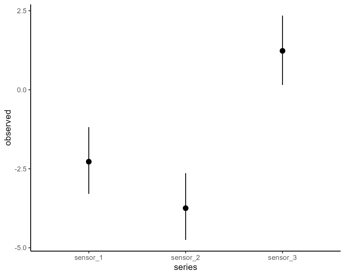'), ask = FALSE)

conditional_effects is simply a wrapper to the more flexible plot_predictions function from the marginaleffects package. We can get more useful plots of these effects using this function for further customisation:

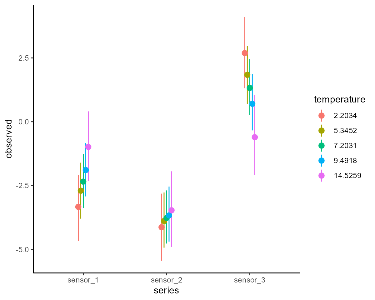
plot_predictions(mod, 
                 condition = c('temperature', 'series', 'series'),
                 points = 0.5) +
  theme(legend.position = 'none')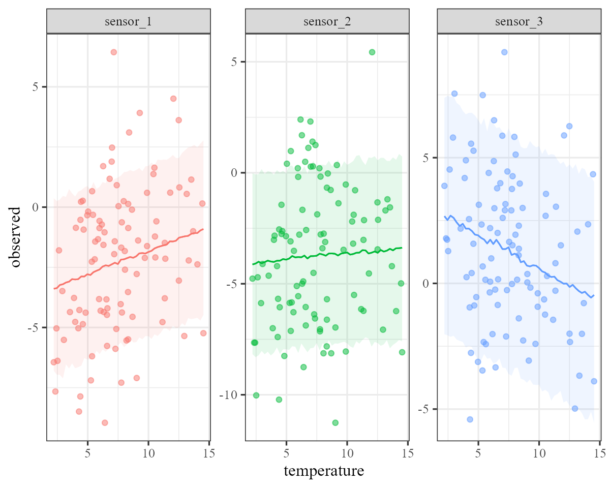

We have successfully estimated effects, some of them nonlinear, that impact the hidden process AND the observations. All in a single joint model. But there can always be challenges with these models, particularly when estimating both process and observation error at the same time. For example, a pairs plot for the observation error for sensor 1 and the hidden process error shows some strong correlations that we might want to deal with by using a more structured prior:

pairs(mod, variable = c('sigma[1]', 'sigma_obs[1]'))

But we will leave the model as-is for this example

Recovering the hidden signal

A final but very key question is whether we can successfully recover the true hidden signal. The trend slot in the returned model parameters has the estimates for this signal, which we can easily plot using the mvgam S3 method for plot. We can also overlay the true values for the hidden signal, which shows that our model has done a good job of recovering it:

plot(mod, type = 'trend')

# Overlay the true simulated signal
points(true_signal, pch = 16, cex = 1, col = 'white')
points(true_signal, pch = 16, cex = 0.8)

Interested in contributing?

I’m actively seeking PhD students and other researchers to work in the areas of ecological forecasting, multivariate model evaluation and development of mvgam. Please reach out if you are interested (n.clark’at’uq.edu.au)

Nicholas J Clark

2024-03-25

The `trend_map` argument

Checking `trend_map` with `run_model = FALSE`

Fitting and inspecting the model

Example: signal detection

The shared signal model

Inspecting effects on both process and observation models

Recovering the hidden signal

Further reading

Interested in contributing?

Shared latent states in mvgam

Nicholas J Clark

2024-03-25

The trend_map argument

Checking trend_map with run_model = FALSE

Fitting and inspecting the model

Example: signal detection

The shared signal model

Inspecting effects on both process and observation models

Recovering the hidden signal

Further reading

Interested in contributing?

The `trend_map` argument

Checking `trend_map` with `run_model = FALSE`