This function allows a previously fitted mvgam model to be updated.
Usage
# S3 method for mvgam
update(
  object,
  formula,
  trend_formula,
  knots,
  trend_knots,
  trend_model,
  family,
  share_obs_params,
  data,
  newdata,
  trend_map,
  use_lv,
  n_lv,
  priors,
  chains,
  burnin,
  samples,
  threads,
  algorithm,
  lfo = FALSE,
  ...
)

# S3 method for jsdgam
update(
  object,
  formula,
  factor_formula,
  knots,
  factor_knots,
  data,
  newdata,
  n_lv,
  family,
  share_obs_params,
  priors,
  chains,
  burnin,
  samples,
  threads,
  algorithm,
  lfo = FALSE,
  ...
)
Arguments
- object
listobject returned frommvgam. Seemvgam()- formula
Optional new
formulaobject. Note,mvgamcurrently does not support dynamic formula updates such as removal of specific terms with- term. When updating, the entire formula needs to be supplied.- trend_formula
An optional
formulaobject specifying the GAM process model formula. If supplied, a linear predictor will be modelled for the latent trends to capture process model evolution separately from the observation model.Important notes:
Should not have a response variable specified on the left-hand side (e.g.,
~ season + s(year))Use
trendinstead ofseriesfor effects that vary across time seriesIn
nmix()family models, sets up linear predictor for latent abundanceConsider dropping one intercept using
- 1convention to avoid estimation challenges
- knots
An optional
listcontaining user specified knot values for basis construction. For most bases the user simply supplies the knots to be used, which must match up with thekvalue supplied. Different terms can use different numbers of knots, unless they share a covariate.- trend_knots
As for
knotsabove, this is an optionallistof knot values for smooth functions within thetrend_formula.- trend_model
characterorfunctionspecifying the time series dynamics for the latent trend.Available options:
None: No latent trend component (GAM component only, likegam)ZMVNorZMVN(): Zero-Mean Multivariate Normal (Stan only)'RW'orRW(): Random Walk'AR1','AR2','AR3'orAR(p = 1, 2, 3): Autoregressive models'CAR1'orCAR(p = 1): Continuous-time AR (Ornstein–Uhlenbeck process)'VAR1'orVAR(): Vector Autoregressive (Stan only)'PWlogistic','PWlinear'orPW(): Piecewise trends (Stan only)'GP'orGP(): Gaussian Process with squared exponential kernel (Stan only)
Additional features:
Moving average and/or correlated process error terms available for most types (e.g.,
RW(cor = TRUE)for multivariate Random Walk)Hierarchical correlations possible for structured data
See mvgam_trends for details and
ZMVN()for examples
- family
familyspecifying the exponential observation family for the series.Supported families:
gaussian(): Real-valued databetar(): Proportional data on(0,1)lognormal(): Non-negative real-valued datastudent_t(): Real-valued dataGamma(): Non-negative real-valued databernoulli(): Binary datapoisson(): Count data (default)nb(): Overdispersed count databinomial(): Count data with imperfect detection when number of trials is known (usecbind()to bind observations and trials)beta_binomial(): Asbinomial()but allows for overdispersionnmix(): Count data with imperfect detection when number of trials is unknown (State-Space N-Mixture model with Poisson latent states and Binomial observations)
See
mvgam_familiesfor more details.- share_obs_params
logical. IfTRUEand thefamilyhas additional family-specific observation parameters (e.g., variance components, dispersion parameters), these will be shared across all outcome variables. Useful when multiple outcomes share properties. Default isFALSE.- data
A
dataframeorlistcontaining the model response variable and covariates required by the GAMformulaand optionaltrend_formula.Required columns for most models:
series: Afactorindex of the series IDs (number of levels should equal number of unique series labels)time:numericorintegerindex of time points. For most dynamic trend types, time should be measured in discrete, regularly spaced intervals (i.e.,c(1, 2, 3, ...)). Irregular spacing is allowed fortrend_model = CAR(1), but zero intervals are adjusted to1e-12to prevent sampling errors.
Special cases:
Models with hierarchical temporal correlation (e.g.,
AR(gr = region, subgr = species)) should NOT include aseriesidentifierModels without temporal dynamics (
trend_model = 'None'ortrend_model = ZMVN()) don't require atimevariable
- newdata
Optional
dataframeorlistof test data containing the same variables as indata. If included, observations in variableywill be set toNAwhen fitting the model so that posterior simulations can be obtained.- trend_map
Optional
data.framespecifying which series should depend on which latent trends. Enables multiple series to depend on the same latent trend process with different observation processes.Required structure:
Column
series: Single unique entry for each series (matching factor levels in data)Column
trend: Integer values indicating which trend each series depends on
Notes:
Sets up latent factor model by enabling
use_lv = TRUEProcess model intercept is NOT automatically suppressed
Not yet supported for continuous time models (
CAR())
- use_lv
logical. IfTRUE, use dynamic factors to estimate series' latent trends in a reduced dimension format. Only available forRW(),AR()andGP()trend models. Default isFALSE. Seelv_correlationsfor examples.- n_lv
integerspecifying the number of latent dynamic factors to use ifuse_lv == TRUE. Cannot exceedn_series. Default ismin(2, floor(n_series / 2)).- priors
An optional
data.framewith prior definitions or, preferably, a vector ofbrmspriorobjects (seeprior()). Seeget_mvgam_priors()and Details for more information.- chains
integerspecifying the number of parallel chains for the model. Ignored for variational inference algorithms.- burnin
integerspecifying the number of warmup iterations to tune sampling algorithms. Ignored for variational inference algorithms.- samples
integerspecifying the number of post-warmup iterations for sampling the posterior distribution.- threads
integer. Experimental option for within-chain parallelisation in Stan usingreduce_sum. Recommended only for experienced Stan users with slow models. Currently works for all families exceptnmix()and when using Cmdstan backend.- algorithm
Character string naming the estimation approach:
"sampling": MCMC (default)"meanfield": Variational inference with factorized normal distributions"fullrank": Variational inference with multivariate normal distribution"laplace": Laplace approximation (cmdstanr only)"pathfinder": Pathfinder algorithm (cmdstanr only)
Can be set globally via
"brms.algorithm"option. Limited testing suggests"meanfield"performs best among non-MCMC approximations for dynamic GAMs.- lfo
logical. Indicates whether this is part of lfo_cv.mvgam call. Returns lighter model version for speed. Users should leave asFALSE.- ...
- factor_formula
Optional new
formulaobject for the factor linear predictors- factor_knots
An optional
listcontaining user specified knot values to be used for basis construction of any smooth terms infactor_formula. For most bases the user simply supplies the knots to be used, which must match up with thekvalue supplied (note that the number of knots is not always justk). Different terms can use different numbers of knots, unless they share a covariate
Value
A list object of class mvgam containing model output,
the text representation of the model file, the mgcv model output (for
easily generating simulations at unsampled covariate values), Dunn-Smyth
residuals for each outcome variable and key information needed for other
functions in the package. See mvgam-class for details. Use
methods(class = "mvgam") for an overview on available methods.
A list object of class mvgam containing model output,
the text representation of the model file, the mgcv model output (for
easily generating simulations at unsampled covariate values), Dunn-Smyth
residuals for each series and key information needed for other functions in
the package. See mvgam-class for details. Use
methods(class = "mvgam") for an overview on available methods.
Examples
# \dontrun{
# Simulate some data and fit a Poisson AR1 model
simdat <- sim_mvgam(n_series = 1, trend_model = AR())
mod <- mvgam(
y ~ s(season, bs = 'cc'),
trend_model = AR(),
noncentred = TRUE,
data = simdat$data_train,
chains = 2
)
#> Compiling Stan program using cmdstanr
#>
#> Start sampling
#> Running MCMC with 2 parallel chains...
#>
#> Chain 1 Iteration: 1 / 1000 [ 0%] (Warmup)
#> Chain 1 Iteration: 100 / 1000 [ 10%] (Warmup)
#> Chain 1 Iteration: 200 / 1000 [ 20%] (Warmup)
#> Chain 1 Iteration: 300 / 1000 [ 30%] (Warmup)
#> Chain 2 Iteration: 1 / 1000 [ 0%] (Warmup)
#> Chain 2 Iteration: 100 / 1000 [ 10%] (Warmup)
#> Chain 1 Iteration: 400 / 1000 [ 40%] (Warmup)
#> Chain 1 Iteration: 500 / 1000 [ 50%] (Warmup)
#> Chain 1 Iteration: 501 / 1000 [ 50%] (Sampling)
#> Chain 1 Iteration: 600 / 1000 [ 60%] (Sampling)
#> Chain 1 Iteration: 700 / 1000 [ 70%] (Sampling)
#> Chain 2 Iteration: 200 / 1000 [ 20%] (Warmup)
#> Chain 2 Iteration: 300 / 1000 [ 30%] (Warmup)
#> Chain 2 Iteration: 400 / 1000 [ 40%] (Warmup)
#> Chain 2 Iteration: 500 / 1000 [ 50%] (Warmup)
#> Chain 2 Iteration: 501 / 1000 [ 50%] (Sampling)
#> Chain 1 Iteration: 800 / 1000 [ 80%] (Sampling)
#> Chain 1 Iteration: 900 / 1000 [ 90%] (Sampling)
#> Chain 2 Iteration: 600 / 1000 [ 60%] (Sampling)
#> Chain 2 Iteration: 700 / 1000 [ 70%] (Sampling)
#> Chain 1 Iteration: 1000 / 1000 [100%] (Sampling)
#> Chain 2 Iteration: 800 / 1000 [ 80%] (Sampling)
#> Chain 2 Iteration: 900 / 1000 [ 90%] (Sampling)
#> Chain 2 Iteration: 1000 / 1000 [100%] (Sampling)
#> Chain 1 finished in 0.4 seconds.
#> Chain 2 finished in 0.4 seconds.
#>
#> Both chains finished successfully.
#> Mean chain execution time: 0.4 seconds.
#> Total execution time: 0.5 seconds.
#>
summary(mod)
#> GAM formula:
#> y ~ s(season, bs = "cc")
#> <environment: 0x5582d0c54f88>
#>
#> Family:
#> poisson
#>
#> Link function:
#> log
#>
#> Trend model:
#> AR()
#>
#> N series:
#> 1
#>
#> N timepoints:
#> 75
#>
#> Status:
#> Fitted using Stan
#> 2 chains, each with iter = 1000; warmup = 500; thin = 1
#> Total post-warmup draws = 1000
#>
#> GAM coefficient (beta) estimates:
#> 2.5% 50% 97.5% Rhat n_eff
#> (Intercept) -1.10 -0.660 -0.30 1 677
#> s(season).1 -0.98 -0.140 0.45 1 638
#> s(season).2 0.71 1.400 2.00 1 755
#> s(season).3 0.87 1.600 2.20 1 585
#> s(season).4 -0.62 0.300 0.97 1 878
#> s(season).5 -1.30 -0.360 0.48 1 1041
#> s(season).6 -1.40 -0.460 0.40 1 1024
#> s(season).7 -0.97 -0.200 0.64 1 1051
#> s(season).8 -0.70 -0.019 0.88 1 630
#>
#> Approximate significance of GAM smooths:
#> edf Ref.df Chi.sq p-value
#> s(season) 5.1 8 39.56 0.00346 **
#> ---
#> Signif. codes: 0 ‘***’ 0.001 ‘**’ 0.01 ‘*’ 0.05 ‘.’ 0.1 ‘ ’ 1
#>
#> standard deviation:
#> 2.5% 50% 97.5% Rhat n_eff
#> sigma[1] 0.1 0.35 0.75 1 338
#>
#> precision parameter:
#> 2.5% 50% 97.5% Rhat n_eff
#> tau[1] 1.8 7.9 96 1 518
#>
#> autoregressive coef 1:
#> 2.5% 50% 97.5% Rhat n_eff
#> ar1[1] -0.96 -0.34 0.84 1 477
#>
#> Stan MCMC diagnostics:
#> ✔ No issues with effective samples per iteration
#> ✔ Rhat looks good for all parameters
#> ✔ No issues with divergences
#> ✔ No issues with maximum tree depth
#>
#> Samples were drawn using sampling(hmc). For each parameter, n_eff is a
#> crude measure of effective sample size, and Rhat is the potential scale
#> reduction factor on split MCMC chains (at convergence, Rhat = 1)
#>
#> Use how_to_cite() to get started describing this model
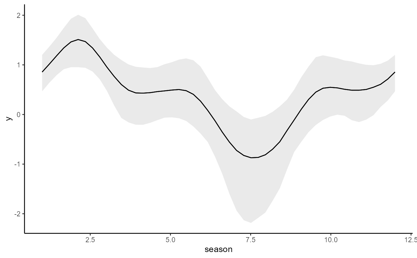
conditional_effects(mod, type = 'link')
 # Update to an AR2 model
updated_mod <- update(
mod,
trend_model = AR(p = 2),
noncentred = TRUE
)
#> Compiling Stan program using cmdstanr
#>
#> Start sampling
#> Running MCMC with 2 parallel chains...
#>
#> Chain 1 Iteration: 1 / 1000 [ 0%] (Warmup)
#> Chain 1 Iteration: 100 / 1000 [ 10%] (Warmup)
#> Chain 1 Iteration: 200 / 1000 [ 20%] (Warmup)
#> Chain 1 Iteration: 300 / 1000 [ 30%] (Warmup)
#> Chain 2 Iteration: 1 / 1000 [ 0%] (Warmup)
#> Chain 2 Iteration: 100 / 1000 [ 10%] (Warmup)
#> Chain 1 Iteration: 400 / 1000 [ 40%] (Warmup)
#> Chain 1 Iteration: 500 / 1000 [ 50%] (Warmup)
#> Chain 1 Iteration: 501 / 1000 [ 50%] (Sampling)
#> Chain 1 Iteration: 600 / 1000 [ 60%] (Sampling)
#> Chain 2 Iteration: 200 / 1000 [ 20%] (Warmup)
#> Chain 2 Iteration: 300 / 1000 [ 30%] (Warmup)
#> Chain 2 Iteration: 400 / 1000 [ 40%] (Warmup)
#> Chain 1 Iteration: 700 / 1000 [ 70%] (Sampling)
#> Chain 1 Iteration: 800 / 1000 [ 80%] (Sampling)
#> Chain 1 Iteration: 900 / 1000 [ 90%] (Sampling)
#> Chain 2 Iteration: 500 / 1000 [ 50%] (Warmup)
#> Chain 2 Iteration: 501 / 1000 [ 50%] (Sampling)
#> Chain 2 Iteration: 600 / 1000 [ 60%] (Sampling)
#> Chain 1 Iteration: 1000 / 1000 [100%] (Sampling)
#> Chain 2 Iteration: 700 / 1000 [ 70%] (Sampling)
#> Chain 2 Iteration: 800 / 1000 [ 80%] (Sampling)
#> Chain 2 Iteration: 900 / 1000 [ 90%] (Sampling)
#> Chain 1 finished in 0.4 seconds.
#> Chain 2 Iteration: 1000 / 1000 [100%] (Sampling)
#> Chain 2 finished in 0.4 seconds.
#>
#> Both chains finished successfully.
#> Mean chain execution time: 0.4 seconds.
#> Total execution time: 0.6 seconds.
#>
summary(updated_mod)
#> GAM formula:
#> y ~ s(season, bs = "cc")
#> <environment: 0x5582d0c54f88>
#>
#> Family:
#> poisson
#>
#> Link function:
#> log
#>
#> Trend model:
#> AR(p = 2)
#>
#> N series:
#> 1
#>
#> N timepoints:
#> 75
#>
#> Status:
#> Fitted using Stan
#> 2 chains, each with iter = 1000; warmup = 500; thin = 1
#> Total post-warmup draws = 1000
#>
#> GAM coefficient (beta) estimates:
#> 2.5% 50% 97.5% Rhat n_eff
#> (Intercept) -1.10 -0.65 -0.33 1.00 467
#> s(season).1 -1.10 -0.10 0.49 1.00 516
#> s(season).2 0.64 1.30 2.10 1.00 430
#> s(season).3 0.87 1.50 2.20 1.00 330
#> s(season).4 -0.54 0.32 1.00 1.00 651
#> s(season).5 -1.20 -0.31 0.40 1.00 530
#> s(season).6 -1.30 -0.42 0.37 1.01 685
#> s(season).7 -1.00 -0.23 0.63 1.00 754
#> s(season).8 -0.73 -0.04 0.90 1.00 505
#>
#> Approximate significance of GAM smooths:
#> edf Ref.df Chi.sq p-value
#> s(season) 2.932 8 51.9 0.0624 .
#> ---
#> Signif. codes: 0 ‘***’ 0.001 ‘**’ 0.01 ‘*’ 0.05 ‘.’ 0.1 ‘ ’ 1
#>
#> standard deviation:
#> 2.5% 50% 97.5% Rhat n_eff
#> sigma[1] 0.1 0.34 0.73 1 212
#>
#> precision parameter:
#> 2.5% 50% 97.5% Rhat n_eff
#> tau[1] 1.9 8.4 92 1 437
#>
#> autoregressive coef 1:
#> 2.5% 50% 97.5% Rhat n_eff
#> ar1[1] -0.95 -0.24 0.85 1.01 251
#>
#> autoregressive coef 2:
#> 2.5% 50% 97.5% Rhat n_eff
#> ar2[1] -0.96 -0.25 0.86 1 260
#>
#> Stan MCMC diagnostics:
#> ✔ No issues with effective samples per iteration
#> ✔ Rhat looks good for all parameters
#> ✔ No issues with divergences
#> ✔ No issues with maximum tree depth
#>
#> Samples were drawn using sampling(hmc). For each parameter, n_eff is a
#> crude measure of effective sample size, and Rhat is the potential scale
#> reduction factor on split MCMC chains (at convergence, Rhat = 1)
#>
#> Use how_to_cite() to get started describing this model
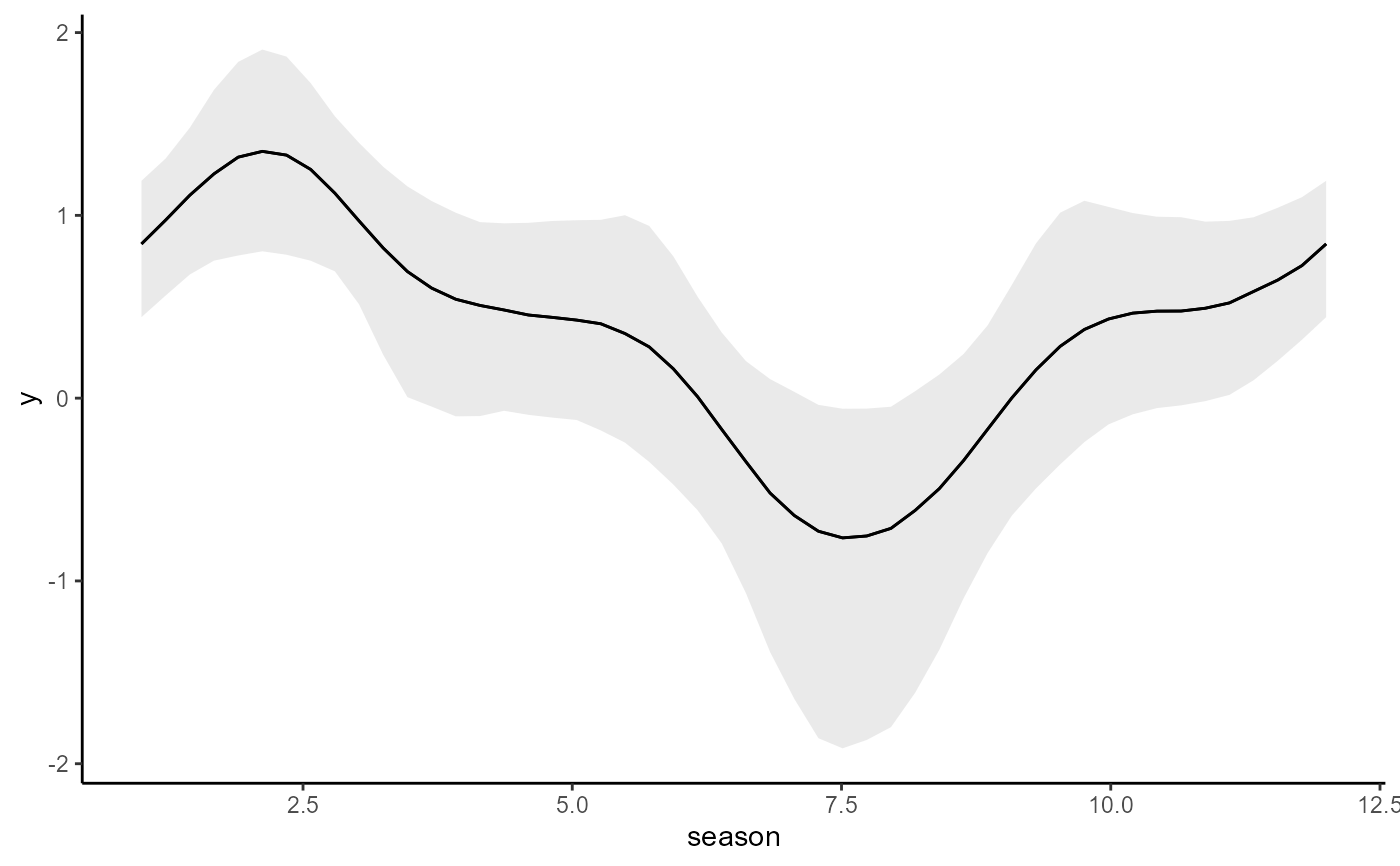
conditional_effects(updated_mod, type = 'link')
# Update to an AR2 model
updated_mod <- update(
mod,
trend_model = AR(p = 2),
noncentred = TRUE
)
#> Compiling Stan program using cmdstanr
#>
#> Start sampling
#> Running MCMC with 2 parallel chains...
#>
#> Chain 1 Iteration: 1 / 1000 [ 0%] (Warmup)
#> Chain 1 Iteration: 100 / 1000 [ 10%] (Warmup)
#> Chain 1 Iteration: 200 / 1000 [ 20%] (Warmup)
#> Chain 1 Iteration: 300 / 1000 [ 30%] (Warmup)
#> Chain 2 Iteration: 1 / 1000 [ 0%] (Warmup)
#> Chain 2 Iteration: 100 / 1000 [ 10%] (Warmup)
#> Chain 1 Iteration: 400 / 1000 [ 40%] (Warmup)
#> Chain 1 Iteration: 500 / 1000 [ 50%] (Warmup)
#> Chain 1 Iteration: 501 / 1000 [ 50%] (Sampling)
#> Chain 1 Iteration: 600 / 1000 [ 60%] (Sampling)
#> Chain 2 Iteration: 200 / 1000 [ 20%] (Warmup)
#> Chain 2 Iteration: 300 / 1000 [ 30%] (Warmup)
#> Chain 2 Iteration: 400 / 1000 [ 40%] (Warmup)
#> Chain 1 Iteration: 700 / 1000 [ 70%] (Sampling)
#> Chain 1 Iteration: 800 / 1000 [ 80%] (Sampling)
#> Chain 1 Iteration: 900 / 1000 [ 90%] (Sampling)
#> Chain 2 Iteration: 500 / 1000 [ 50%] (Warmup)
#> Chain 2 Iteration: 501 / 1000 [ 50%] (Sampling)
#> Chain 2 Iteration: 600 / 1000 [ 60%] (Sampling)
#> Chain 1 Iteration: 1000 / 1000 [100%] (Sampling)
#> Chain 2 Iteration: 700 / 1000 [ 70%] (Sampling)
#> Chain 2 Iteration: 800 / 1000 [ 80%] (Sampling)
#> Chain 2 Iteration: 900 / 1000 [ 90%] (Sampling)
#> Chain 1 finished in 0.4 seconds.
#> Chain 2 Iteration: 1000 / 1000 [100%] (Sampling)
#> Chain 2 finished in 0.4 seconds.
#>
#> Both chains finished successfully.
#> Mean chain execution time: 0.4 seconds.
#> Total execution time: 0.6 seconds.
#>
summary(updated_mod)
#> GAM formula:
#> y ~ s(season, bs = "cc")
#> <environment: 0x5582d0c54f88>
#>
#> Family:
#> poisson
#>
#> Link function:
#> log
#>
#> Trend model:
#> AR(p = 2)
#>
#> N series:
#> 1
#>
#> N timepoints:
#> 75
#>
#> Status:
#> Fitted using Stan
#> 2 chains, each with iter = 1000; warmup = 500; thin = 1
#> Total post-warmup draws = 1000
#>
#> GAM coefficient (beta) estimates:
#> 2.5% 50% 97.5% Rhat n_eff
#> (Intercept) -1.10 -0.65 -0.33 1.00 467
#> s(season).1 -1.10 -0.10 0.49 1.00 516
#> s(season).2 0.64 1.30 2.10 1.00 430
#> s(season).3 0.87 1.50 2.20 1.00 330
#> s(season).4 -0.54 0.32 1.00 1.00 651
#> s(season).5 -1.20 -0.31 0.40 1.00 530
#> s(season).6 -1.30 -0.42 0.37 1.01 685
#> s(season).7 -1.00 -0.23 0.63 1.00 754
#> s(season).8 -0.73 -0.04 0.90 1.00 505
#>
#> Approximate significance of GAM smooths:
#> edf Ref.df Chi.sq p-value
#> s(season) 2.932 8 51.9 0.0624 .
#> ---
#> Signif. codes: 0 ‘***’ 0.001 ‘**’ 0.01 ‘*’ 0.05 ‘.’ 0.1 ‘ ’ 1
#>
#> standard deviation:
#> 2.5% 50% 97.5% Rhat n_eff
#> sigma[1] 0.1 0.34 0.73 1 212
#>
#> precision parameter:
#> 2.5% 50% 97.5% Rhat n_eff
#> tau[1] 1.9 8.4 92 1 437
#>
#> autoregressive coef 1:
#> 2.5% 50% 97.5% Rhat n_eff
#> ar1[1] -0.95 -0.24 0.85 1.01 251
#>
#> autoregressive coef 2:
#> 2.5% 50% 97.5% Rhat n_eff
#> ar2[1] -0.96 -0.25 0.86 1 260
#>
#> Stan MCMC diagnostics:
#> ✔ No issues with effective samples per iteration
#> ✔ Rhat looks good for all parameters
#> ✔ No issues with divergences
#> ✔ No issues with maximum tree depth
#>
#> Samples were drawn using sampling(hmc). For each parameter, n_eff is a
#> crude measure of effective sample size, and Rhat is the potential scale
#> reduction factor on split MCMC chains (at convergence, Rhat = 1)
#>
#> Use how_to_cite() to get started describing this model
conditional_effects(updated_mod, type = 'link')
 # Now update to a Binomial AR1 by adding information on trials
# requires that we supply newdata that contains the 'trials' variable
simdat$data_train$trials <- max(simdat$data_train$y) + 15
updated_mod <- update(
mod,
formula = cbind(y, trials) ~ s(season, bs = 'cc'),
noncentred = TRUE,
data = simdat$data_train,
family = binomial()
)
#> Compiling Stan program using cmdstanr
#>
#> Start sampling
#> Running MCMC with 2 parallel chains...
#>
#> Chain 1 Iteration: 1 / 1000 [ 0%] (Warmup)
#> Chain 1 Iteration: 100 / 1000 [ 10%] (Warmup)
#> Chain 1 Iteration: 200 / 1000 [ 20%] (Warmup)
#> Chain 1 Iteration: 300 / 1000 [ 30%] (Warmup)
#> Chain 1 Iteration: 400 / 1000 [ 40%] (Warmup)
#> Chain 2 Iteration: 1 / 1000 [ 0%] (Warmup)
#> Chain 2 Iteration: 100 / 1000 [ 10%] (Warmup)
#> Chain 2 Iteration: 200 / 1000 [ 20%] (Warmup)
#> Chain 1 Iteration: 500 / 1000 [ 50%] (Warmup)
#> Chain 1 Iteration: 501 / 1000 [ 50%] (Sampling)
#> Chain 1 Iteration: 600 / 1000 [ 60%] (Sampling)
#> Chain 1 Iteration: 700 / 1000 [ 70%] (Sampling)
#> Chain 1 Iteration: 800 / 1000 [ 80%] (Sampling)
#> Chain 2 Iteration: 300 / 1000 [ 30%] (Warmup)
#> Chain 2 Iteration: 400 / 1000 [ 40%] (Warmup)
#> Chain 2 Iteration: 500 / 1000 [ 50%] (Warmup)
#> Chain 2 Iteration: 501 / 1000 [ 50%] (Sampling)
#> Chain 1 Iteration: 900 / 1000 [ 90%] (Sampling)
#> Chain 1 Iteration: 1000 / 1000 [100%] (Sampling)
#> Chain 2 Iteration: 600 / 1000 [ 60%] (Sampling)
#> Chain 2 Iteration: 700 / 1000 [ 70%] (Sampling)
#> Chain 2 Iteration: 800 / 1000 [ 80%] (Sampling)
#> Chain 1 finished in 0.4 seconds.
#> Chain 2 Iteration: 900 / 1000 [ 90%] (Sampling)
#> Chain 2 Iteration: 1000 / 1000 [100%] (Sampling)
#> Chain 2 finished in 0.5 seconds.
#>
#> Both chains finished successfully.
#> Mean chain execution time: 0.4 seconds.
#> Total execution time: 0.6 seconds.
#>
summary(updated_mod)
#> GAM formula:
#> cbind(y, trials) ~ s(season, bs = "cc")
#> <environment: 0x5582d0c54f88>
#>
#> Family:
#> binomial
#>
#> Link function:
#> logit
#>
#> Trend model:
#> AR()
#>
#> N series:
#> 1
#>
#> N timepoints:
#> 75
#>
#> Status:
#> Fitted using Stan
#> 2 chains, each with iter = 1000; warmup = 500; thin = 1
#> Total post-warmup draws = 1000
#>
#> GAM coefficient (beta) estimates:
#> 2.5% 50% 97.5% Rhat n_eff
#> (Intercept) -4.10 -3.700 -3.40 1 782
#> s(season).1 -1.10 -0.170 0.51 1 557
#> s(season).2 0.77 1.400 2.10 1 702
#> s(season).3 0.97 1.700 2.40 1 585
#> s(season).4 -0.60 0.290 1.00 1 1025
#> s(season).5 -1.30 -0.360 0.43 1 964
#> s(season).6 -1.30 -0.480 0.37 1 906
#> s(season).7 -1.10 -0.190 0.60 1 862
#> s(season).8 -0.73 0.051 0.94 1 598
#>
#> Approximate significance of GAM smooths:
#> edf Ref.df Chi.sq p-value
#> s(season) 4.023 8 46.68 0.00311 **
#> ---
#> Signif. codes: 0 ‘***’ 0.001 ‘**’ 0.01 ‘*’ 0.05 ‘.’ 0.1 ‘ ’ 1
#>
#> standard deviation:
#> 2.5% 50% 97.5% Rhat n_eff
#> sigma[1] 0.11 0.39 0.85 1 338
#>
#> precision parameter:
#> 2.5% 50% 97.5% Rhat n_eff
#> tau[1] 1.4 6.7 76 1 603
#>
#> autoregressive coef 1:
#> 2.5% 50% 97.5% Rhat n_eff
#> ar1[1] -0.96 -0.35 0.81 1 460
#>
#> Stan MCMC diagnostics:
#> ✔ No issues with effective samples per iteration
#> ✔ Rhat looks good for all parameters
#> ✔ No issues with divergences
#> ✔ No issues with maximum tree depth
#>
#> Samples were drawn using sampling(hmc). For each parameter, n_eff is a
#> crude measure of effective sample size, and Rhat is the potential scale
#> reduction factor on split MCMC chains (at convergence, Rhat = 1)
#>
#> Use how_to_cite() to get started describing this model
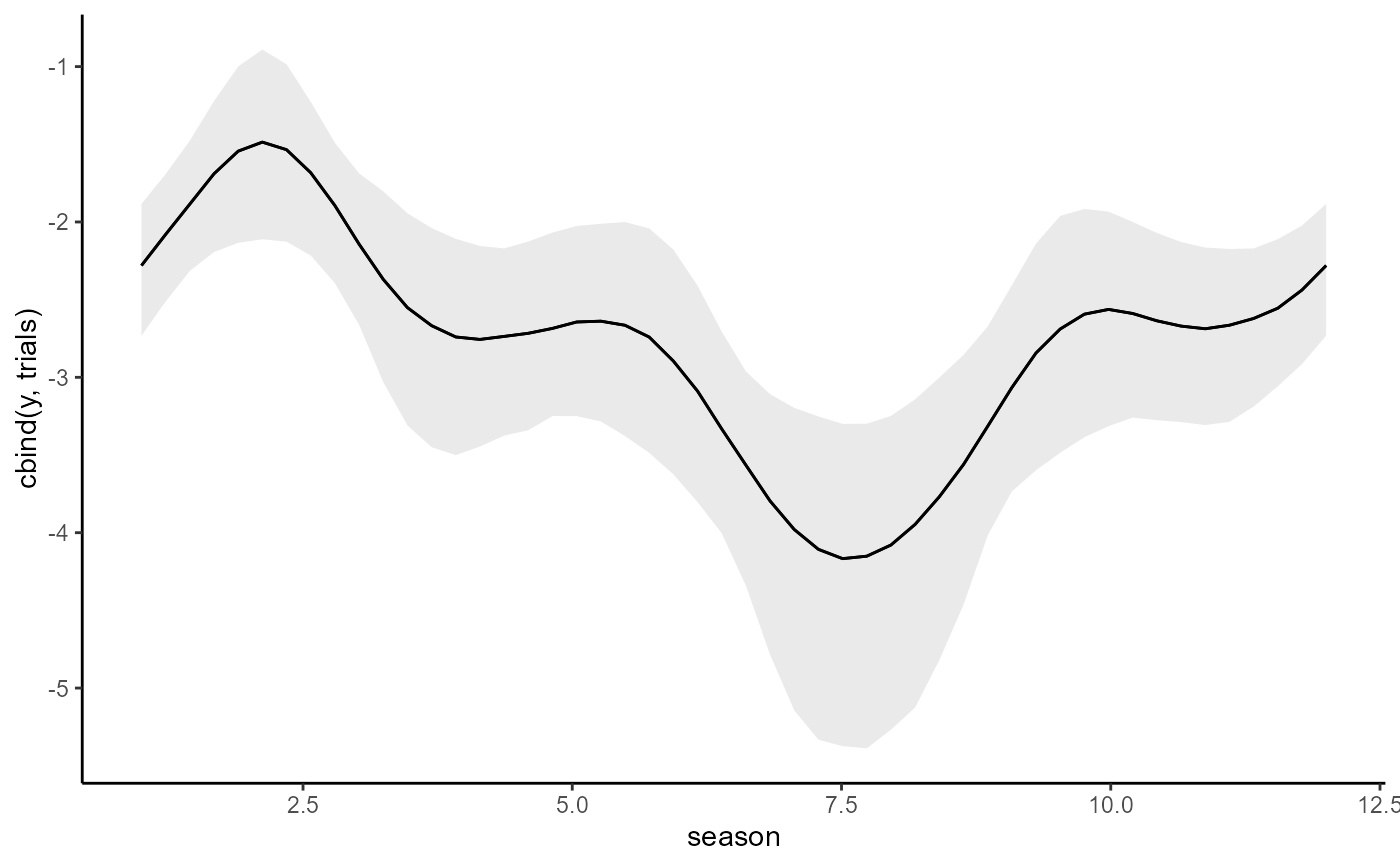
conditional_effects(updated_mod, type = 'link')
# Now update to a Binomial AR1 by adding information on trials
# requires that we supply newdata that contains the 'trials' variable
simdat$data_train$trials <- max(simdat$data_train$y) + 15
updated_mod <- update(
mod,
formula = cbind(y, trials) ~ s(season, bs = 'cc'),
noncentred = TRUE,
data = simdat$data_train,
family = binomial()
)
#> Compiling Stan program using cmdstanr
#>
#> Start sampling
#> Running MCMC with 2 parallel chains...
#>
#> Chain 1 Iteration: 1 / 1000 [ 0%] (Warmup)
#> Chain 1 Iteration: 100 / 1000 [ 10%] (Warmup)
#> Chain 1 Iteration: 200 / 1000 [ 20%] (Warmup)
#> Chain 1 Iteration: 300 / 1000 [ 30%] (Warmup)
#> Chain 1 Iteration: 400 / 1000 [ 40%] (Warmup)
#> Chain 2 Iteration: 1 / 1000 [ 0%] (Warmup)
#> Chain 2 Iteration: 100 / 1000 [ 10%] (Warmup)
#> Chain 2 Iteration: 200 / 1000 [ 20%] (Warmup)
#> Chain 1 Iteration: 500 / 1000 [ 50%] (Warmup)
#> Chain 1 Iteration: 501 / 1000 [ 50%] (Sampling)
#> Chain 1 Iteration: 600 / 1000 [ 60%] (Sampling)
#> Chain 1 Iteration: 700 / 1000 [ 70%] (Sampling)
#> Chain 1 Iteration: 800 / 1000 [ 80%] (Sampling)
#> Chain 2 Iteration: 300 / 1000 [ 30%] (Warmup)
#> Chain 2 Iteration: 400 / 1000 [ 40%] (Warmup)
#> Chain 2 Iteration: 500 / 1000 [ 50%] (Warmup)
#> Chain 2 Iteration: 501 / 1000 [ 50%] (Sampling)
#> Chain 1 Iteration: 900 / 1000 [ 90%] (Sampling)
#> Chain 1 Iteration: 1000 / 1000 [100%] (Sampling)
#> Chain 2 Iteration: 600 / 1000 [ 60%] (Sampling)
#> Chain 2 Iteration: 700 / 1000 [ 70%] (Sampling)
#> Chain 2 Iteration: 800 / 1000 [ 80%] (Sampling)
#> Chain 1 finished in 0.4 seconds.
#> Chain 2 Iteration: 900 / 1000 [ 90%] (Sampling)
#> Chain 2 Iteration: 1000 / 1000 [100%] (Sampling)
#> Chain 2 finished in 0.5 seconds.
#>
#> Both chains finished successfully.
#> Mean chain execution time: 0.4 seconds.
#> Total execution time: 0.6 seconds.
#>
summary(updated_mod)
#> GAM formula:
#> cbind(y, trials) ~ s(season, bs = "cc")
#> <environment: 0x5582d0c54f88>
#>
#> Family:
#> binomial
#>
#> Link function:
#> logit
#>
#> Trend model:
#> AR()
#>
#> N series:
#> 1
#>
#> N timepoints:
#> 75
#>
#> Status:
#> Fitted using Stan
#> 2 chains, each with iter = 1000; warmup = 500; thin = 1
#> Total post-warmup draws = 1000
#>
#> GAM coefficient (beta) estimates:
#> 2.5% 50% 97.5% Rhat n_eff
#> (Intercept) -4.10 -3.700 -3.40 1 782
#> s(season).1 -1.10 -0.170 0.51 1 557
#> s(season).2 0.77 1.400 2.10 1 702
#> s(season).3 0.97 1.700 2.40 1 585
#> s(season).4 -0.60 0.290 1.00 1 1025
#> s(season).5 -1.30 -0.360 0.43 1 964
#> s(season).6 -1.30 -0.480 0.37 1 906
#> s(season).7 -1.10 -0.190 0.60 1 862
#> s(season).8 -0.73 0.051 0.94 1 598
#>
#> Approximate significance of GAM smooths:
#> edf Ref.df Chi.sq p-value
#> s(season) 4.023 8 46.68 0.00311 **
#> ---
#> Signif. codes: 0 ‘***’ 0.001 ‘**’ 0.01 ‘*’ 0.05 ‘.’ 0.1 ‘ ’ 1
#>
#> standard deviation:
#> 2.5% 50% 97.5% Rhat n_eff
#> sigma[1] 0.11 0.39 0.85 1 338
#>
#> precision parameter:
#> 2.5% 50% 97.5% Rhat n_eff
#> tau[1] 1.4 6.7 76 1 603
#>
#> autoregressive coef 1:
#> 2.5% 50% 97.5% Rhat n_eff
#> ar1[1] -0.96 -0.35 0.81 1 460
#>
#> Stan MCMC diagnostics:
#> ✔ No issues with effective samples per iteration
#> ✔ Rhat looks good for all parameters
#> ✔ No issues with divergences
#> ✔ No issues with maximum tree depth
#>
#> Samples were drawn using sampling(hmc). For each parameter, n_eff is a
#> crude measure of effective sample size, and Rhat is the potential scale
#> reduction factor on split MCMC chains (at convergence, Rhat = 1)
#>
#> Use how_to_cite() to get started describing this model
conditional_effects(updated_mod, type = 'link')
 # }
# }