This function sets up a Joint Species Distribution Model whereby the residual associations among species can be modelled in a reduced-rank format using a set of latent factors. The factor specification is extremely flexible, allowing users to include spatial, temporal or any other type of predictor effects to more efficiently capture unmodelled residual associations, while the observation model can also be highly flexible (including all smooth, GP and other effects that mvgam can handle)
Usage
jsdgam(
  formula,
  factor_formula = ~-1,
  knots,
  factor_knots,
  data,
  newdata,
  family = poisson(),
  unit = time,
  species = series,
  share_obs_params = FALSE,
  priors,
  n_lv = 2,
  backend = getOption("brms.backend", "cmdstanr"),
  algorithm = getOption("brms.algorithm", "sampling"),
  control = list(max_treedepth = 10, adapt_delta = 0.8),
  chains = 4,
  burnin = 500,
  samples = 500,
  thin = 1,
  parallel = TRUE,
  threads = 1,
  silent = 1,
  run_model = TRUE,
  return_model_data = FALSE,
  residuals = TRUE,
  ...
)
Arguments
- formula
A
formulaobject specifying the GAM observation model formula. These are exactly like the formula for a GLM except that smooth terms,s(),te(),ti(),t2(), as well as time-varyingdynamic()terms, nonparametricgp()terms and offsets usingoffset(), can be added to the right hand side to specify that the linear predictor depends on smooth functions of predictors (or linear functionals of these). Details of the formula syntax used by mvgam can be found inmvgam_formulae- factor_formula
A
formulaobject specifying the linear predictor effects for the latent factors. Useby = trendwithin calls to functional terms (i.e.s(),te(),ti(),t2(),dynamic(), orgp()) to ensure that each factor captures a different axis of variation. See the example below as an illustration- knots
An optional
listcontaining user specified knot values for basis construction. For most bases the user simply supplies the knots to be used, which must match up with thekvalue supplied. Different terms can use different numbers of knots, unless they share a covariate.- factor_knots
An optional
listcontaining user specified knot values to be used for basis construction of any smooth terms infactor_formula. For most bases the user simply supplies the knots to be used, which must match up with thekvalue supplied (note that the number of knots is not always justk). Different terms can use different numbers of knots, unless they share a covariate- data
A
dataframeorlistcontaining the model response variable and covariates required by the GAMformulaandfactor_formulaobjects- newdata
Optional
dataframeorlistof test data containing the same variables as indata. If included, observations in variableywill be set toNAwhen fitting the model so that posterior simulations can be obtained.- family
familyspecifying the observation family for the outcomes. Currently supported families are:gaussian()for real-valued databetar()for proportional data on(0,1)lognormal()for non-negative real-valued datastudent_t()for real-valued dataGamma()for non-negative real-valued databernoulli()for binary datapoisson()for count datanb()for overdispersed count databinomial()for count data with imperfect detection when the number of trials is known; note that thecbind()function must be used to bind the discrete observations and the discrete number of trialsbeta_binomial()as forbinomial()but allows for overdispersion
Default is
poisson(). Seemvgam_familiesfor more details- unit
The unquoted name of the variable that represents the unit of analysis in
dataover which latent residuals should be correlated. This variable should be either anumericorintegervariable in the supplieddata. Defaults totimeto be consistent with other functionalities in mvgam, though note that the data need not be time series in this case. See examples below for further details and explanations- species
The unquoted name of the
factorvariable that indexes the different response units indata(usually'species'in a JSDM). Defaults toseriesto be consistent with othermvgammodels- share_obs_params
logical. IfTRUEand thefamilyhas additional family-specific observation parameters (e.g., variance components, dispersion parameters), these will be shared across all outcome variables. Useful when multiple outcomes share properties. Default isFALSE.- priors
An optional
data.framewith prior definitions (in Stan syntax) or, preferentially, a vector containing objects of classbrmsprior(see.priorfor details). See get_mvgam_priors and for more information on changing default prior distributions- n_lv
integerthe number of latent factors to use for modelling residual associations. Cannot be> n_species. Defaults arbitrarily to2- backend
Character string naming the package for Stan model fitting. Options are
"cmdstanr"(default) or"rstan". Can be set globally via"brms.backend"option. See https://mc-stan.org/rstan/ and https://mc-stan.org/cmdstanr/ for details.- algorithm
Character string naming the estimation approach:
"sampling": MCMC (default)"meanfield": Variational inference with factorized normal distributions"fullrank": Variational inference with multivariate normal distribution"laplace": Laplace approximation (cmdstanr only)"pathfinder": Pathfinder algorithm (cmdstanr only)
Can be set globally via
"brms.algorithm"option. Limited testing suggests"meanfield"performs best among non-MCMC approximations for dynamic GAMs.- control
Named
listfor controlling sampler behaviour. Valid elements includemax_treedepth,adapt_deltaandinit.- chains
integerspecifying the number of parallel chains for the model. Ignored for variational inference algorithms.- burnin
integerspecifying the number of warmup iterations to tune sampling algorithms. Ignored for variational inference algorithms.- samples
integerspecifying the number of post-warmup iterations for sampling the posterior distribution.- thin
Thinning interval for monitors. Ignored for variational inference algorithms.
- parallel
logicalspecifying whether to use multiple cores for parallel MCMC simulation. IfTRUE, usesmin(c(chains, parallel::detectCores() - 1))cores.- threads
integerExperimental option to use multithreading for within-chain parallelisation inStan. We recommend its use only if you are experienced withStan'sreduce_sumfunction and have a slow running model that cannot be sped up by any other means. Currently works for all families when using cmdstanr as the backend- silent
Verbosity level between
0and2. If1(default), most informational messages are suppressed. If2, even more messages are suppressed. Sampling progress is still printed - setrefresh = 0to disable. Forbackend = "rstan", also setopen_progress = FALSEto prevent additional progress bars.- run_model
logical. IfFALSE, the model is not fitted but instead the function returns the model file and the data/initial values needed to fit the model outside ofmvgam.- return_model_data
logical. IfTRUE, the list of data needed to fit the model is returned, along with initial values for smooth and AR parameters, once the model is fitted. Helpful for users who wish to modify the model file to add other stochastic elements. Default isFALSEunlessrun_model == FALSE.- residuals
logical. Whether to compute series-level randomized quantile residuals. Default isTRUE. Set toFALSEto save time and reduce object size (can add later using add_residuals).- ...
Other arguments to pass to mvgam
Value
A list object of class mvgam containing model output,
the text representation of the model file, the mgcv model output (for easily
generating simulations at unsampled covariate values), Dunn-Smyth residuals
for each species and key information needed for other functions in the
package. See mvgam-class for details. Use
methods(class = "mvgam") for an overview on available methods
Details
Joint Species Distribution Models allow for responses of multiple
species to be learned hierarchically, whereby responses to environmental
variables in formula can be partially pooled and any latent, unmodelled
residual associations can also be learned. In mvgam, both of these
effects can be modelled with the full power of latent factor Hierarchical
GAMs, providing unmatched flexibility to model full communities of species.
When calling jsdgam, an initial State-Space model using trend = 'None' is
set up and then modified to include the latent factors and their linear
predictors. Consequently, you can inspect priors for these models using
get_mvgam_priors by supplying the relevant formula, factor_formula,
data and family arguments and keeping the default trend = 'None'.
In a JSDGAM, the expectation of response \(Y_{ij}\) is modelled with
$$g(\mu_{ij}) = X_i\beta + u_i\theta_j,$$
where \(g(.)\) is a known link function,
\(X\) is a design matrix of linear predictors (with associated \(\beta\)
coefficients), \(u\) are \(n_{lv}\)-variate latent factors
(\(n_{lv}\)<<\(n_{species}\)) and \(\theta_j\) are species-specific
loadings on the latent factors, respectively. The design matrix \(X\) and
\(\beta\) coefficients are constructed and modelled using formula and
can contain any of mvgam's predictor effects, including random intercepts
and slopes, multidimensional penalized smooths, GP effects etc... The factor
loadings \(\theta_j\) are constrained for identifiability but can be used
to reconstruct an estimate of the species' residual variance-covariance
matrix using \(\Theta \Theta'\) (see the example below and
residual_cor() for details). The latent factors are further modelled using:
$$
u_i \sim \text{Normal}(Q_i\beta_{factor}, 1)
$$
where the second design matrix \(Q\) and associated \(\beta_{factor}\)
coefficients are constructed and modelled using factor_formula. Again, the
effects that make up this linear predictor can contain any of mvgam's
allowed predictor effects, providing enormous flexibility for modelling
species' communities.
References
Nicholas J Clark & Konstans Wells (2023). Dynamic generalised
additive models (DGAMs) for forecasting discrete ecological time series.
Methods in Ecology and Evolution. 14:3, 771-784.
David I Warton, F Guillaume Blanchet, Robert B O'Hara, Otso Ovaskainen, Sara
Taskinen, Steven C Walker & Francis KC Hui (2015). So many variables: joint
modeling in community ecology. Trends in Ecology & Evolution 30:12, 766-779.
Examples
# \dontrun{
# ========================================================================
# Example 1: Basic JSDGAM with Portal Data
# ========================================================================
# Fit a JSDGAM to the portal_data captures
mod <- jsdgam(
formula = captures ~
# Fixed effects of NDVI and mintemp, row effect as a GP of time
ndvi_ma12:series + mintemp:series + gp(time, k = 15),
factor_formula = ~ -1,
data = portal_data,
unit = time,
species = series,
family = poisson(),
n_lv = 2,
silent = 2,
chains = 2
)
# Plot covariate effects
library(ggplot2); theme_set(theme_bw())
plot_predictions(
mod,
condition = c('ndvi_ma12', 'series', 'series')
)
 plot_predictions(
mod,
condition = c('mintemp', 'series', 'series')
)
plot_predictions(
mod,
condition = c('mintemp', 'series', 'series')
)
 # A residual correlation plot
plot(residual_cor(mod))
# A residual correlation plot
plot(residual_cor(mod))
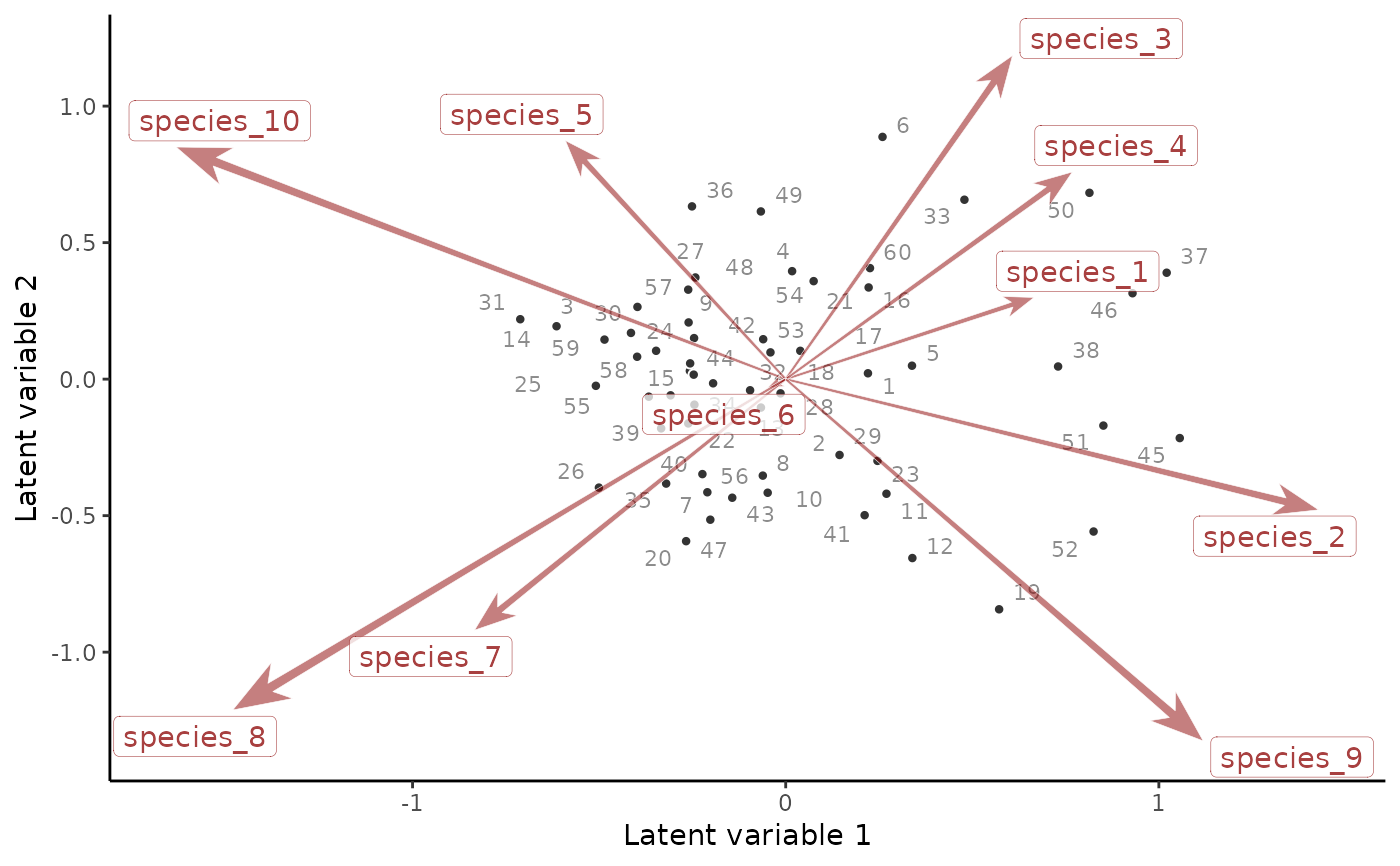
 # An ordination biplot can also be constructed
# from the factor scores and their loadings
if(requireNamespace('ggrepel', quietly = TRUE)){
ordinate(mod, alpha = 0.7)
}
#> Registered S3 methods overwritten by 'ggpp':
#> method from
#> heightDetails.titleGrob ggplot2
#> widthDetails.titleGrob ggplot2
#> Warning: ggrepel: 1 unlabeled data points (too many overlaps). Consider increasing max.overlaps
# An ordination biplot can also be constructed
# from the factor scores and their loadings
if(requireNamespace('ggrepel', quietly = TRUE)){
ordinate(mod, alpha = 0.7)
}
#> Registered S3 methods overwritten by 'ggpp':
#> method from
#> heightDetails.titleGrob ggplot2
#> widthDetails.titleGrob ggplot2
#> Warning: ggrepel: 1 unlabeled data points (too many overlaps). Consider increasing max.overlaps
 # ========================================================================
# Example 2: Advanced JSDGAM with Spatial Predictors
# ========================================================================
# Simulate latent count data for 500 spatial locations and 10 species
set.seed(0)
N_points <- 500
N_species <- 10
# Species-level intercepts (on the log scale)
alphas <- runif(N_species, 2, 2.25)
# Simulate a covariate and species-level responses to it
temperature <- rnorm(N_points)
betas <- runif(N_species, -0.5, 0.5)
# Simulate points uniformly over a space
lon <- runif(N_points, min = 150, max = 155)
lat <- runif(N_points, min = -20, max = -19)
# Set up spatial basis functions as a tensor product of lat and lon
sm <- mgcv::smoothCon(
mgcv::te(lon, lat, k = 5),
data = data.frame(lon, lat),
knots = NULL
)[[1]]
# The design matrix for this smooth is in the 'X' slot
des_mat <- sm$X
dim(des_mat)
#> [1] 500 25
# Function to generate a random covariance matrix where all variables
# have unit variance (i.e. diagonals are all 1)
random_Sigma = function(N){
L_Omega <- matrix(0, N, N);
L_Omega[1, 1] <- 1;
for (i in 2 : N) {
bound <- 1;
for (j in 1 : (i - 1)) {
L_Omega[i, j] <- runif(1, -sqrt(bound), sqrt(bound));
bound <- bound - L_Omega[i, j] ^ 2;
}
L_Omega[i, i] <- sqrt(bound);
}
Sigma <- L_Omega %*% t(L_Omega);
return(Sigma)
}
# Simulate a variance-covariance matrix for the correlations among
# basis coefficients
Sigma <- random_Sigma(N = NCOL(des_mat))
# Now simulate the species-level basis coefficients hierarchically, where
# spatial basis function correlations are a convex sum of a base correlation
# matrix and a species-level correlation matrix
basis_coefs <- matrix(NA, nrow = N_species, ncol = NCOL(Sigma))
base_field <- mgcv::rmvn(1, mu = rep(0, NCOL(Sigma)), V = Sigma)
for(t in 1:N_species){
corOmega <- (cov2cor(Sigma) * 0.7) +
(0.3 * cov2cor(random_Sigma(N = NCOL(des_mat))))
basis_coefs[t, ] <- mgcv::rmvn(1, mu = rep(0, NCOL(Sigma)), V = corOmega)
}
# Simulate the latent spatial processes
st_process <- do.call(rbind, lapply(seq_len(N_species), function(t){
data.frame(
lat = lat,
lon = lon,
species = paste0('species_', t),
temperature = temperature,
process = alphas[t] +
betas[t] * temperature +
des_mat %*% basis_coefs[t,]
)
}))
# Now take noisy observations at some of the points (60)
obs_points <- sample(1:N_points, size = 60, replace = FALSE)
obs_points <- data.frame(
lat = lat[obs_points],
lon = lon[obs_points],
site = 1:60
)
# Keep only the process data at these points
st_process %>%
dplyr::inner_join(obs_points, by = c('lat', 'lon')) %>%
# now take noisy Poisson observations of the process
dplyr::mutate(count = rpois(NROW(.), lambda = exp(process))) %>%
dplyr::mutate(species = factor(
species,
levels = paste0('species_', 1:N_species)
)) %>%
dplyr::group_by(lat, lon) -> dat
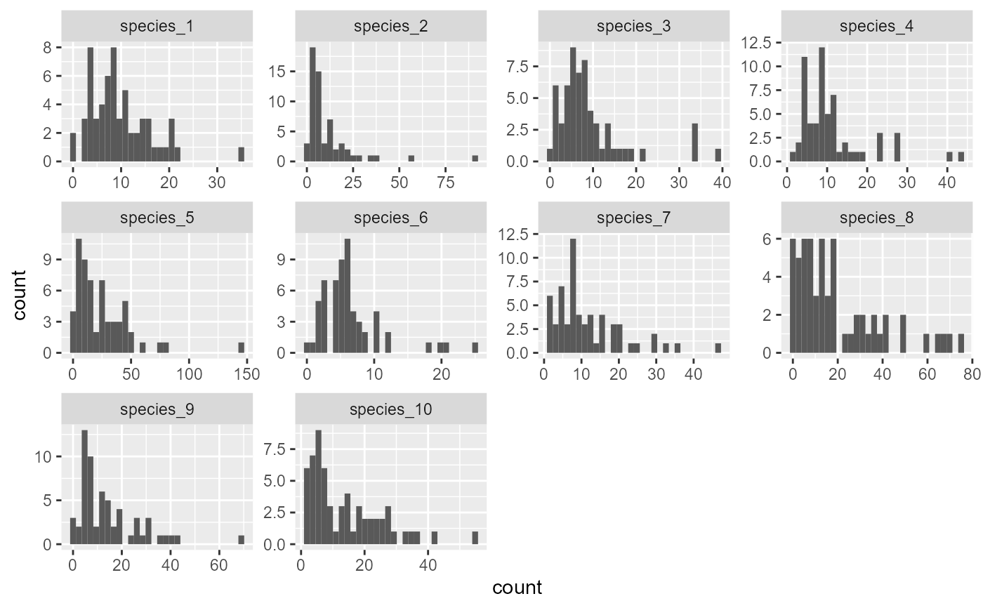
# View the count distributions for each species
ggplot(dat, aes(x = count)) +
geom_histogram() +
facet_wrap(~ species, scales = 'free')
#> `stat_bin()` using `bins = 30`. Pick better value `binwidth`.
# ========================================================================
# Example 2: Advanced JSDGAM with Spatial Predictors
# ========================================================================
# Simulate latent count data for 500 spatial locations and 10 species
set.seed(0)
N_points <- 500
N_species <- 10
# Species-level intercepts (on the log scale)
alphas <- runif(N_species, 2, 2.25)
# Simulate a covariate and species-level responses to it
temperature <- rnorm(N_points)
betas <- runif(N_species, -0.5, 0.5)
# Simulate points uniformly over a space
lon <- runif(N_points, min = 150, max = 155)
lat <- runif(N_points, min = -20, max = -19)
# Set up spatial basis functions as a tensor product of lat and lon
sm <- mgcv::smoothCon(
mgcv::te(lon, lat, k = 5),
data = data.frame(lon, lat),
knots = NULL
)[[1]]
# The design matrix for this smooth is in the 'X' slot
des_mat <- sm$X
dim(des_mat)
#> [1] 500 25
# Function to generate a random covariance matrix where all variables
# have unit variance (i.e. diagonals are all 1)
random_Sigma = function(N){
L_Omega <- matrix(0, N, N);
L_Omega[1, 1] <- 1;
for (i in 2 : N) {
bound <- 1;
for (j in 1 : (i - 1)) {
L_Omega[i, j] <- runif(1, -sqrt(bound), sqrt(bound));
bound <- bound - L_Omega[i, j] ^ 2;
}
L_Omega[i, i] <- sqrt(bound);
}
Sigma <- L_Omega %*% t(L_Omega);
return(Sigma)
}
# Simulate a variance-covariance matrix for the correlations among
# basis coefficients
Sigma <- random_Sigma(N = NCOL(des_mat))
# Now simulate the species-level basis coefficients hierarchically, where
# spatial basis function correlations are a convex sum of a base correlation
# matrix and a species-level correlation matrix
basis_coefs <- matrix(NA, nrow = N_species, ncol = NCOL(Sigma))
base_field <- mgcv::rmvn(1, mu = rep(0, NCOL(Sigma)), V = Sigma)
for(t in 1:N_species){
corOmega <- (cov2cor(Sigma) * 0.7) +
(0.3 * cov2cor(random_Sigma(N = NCOL(des_mat))))
basis_coefs[t, ] <- mgcv::rmvn(1, mu = rep(0, NCOL(Sigma)), V = corOmega)
}
# Simulate the latent spatial processes
st_process <- do.call(rbind, lapply(seq_len(N_species), function(t){
data.frame(
lat = lat,
lon = lon,
species = paste0('species_', t),
temperature = temperature,
process = alphas[t] +
betas[t] * temperature +
des_mat %*% basis_coefs[t,]
)
}))
# Now take noisy observations at some of the points (60)
obs_points <- sample(1:N_points, size = 60, replace = FALSE)
obs_points <- data.frame(
lat = lat[obs_points],
lon = lon[obs_points],
site = 1:60
)
# Keep only the process data at these points
st_process %>%
dplyr::inner_join(obs_points, by = c('lat', 'lon')) %>%
# now take noisy Poisson observations of the process
dplyr::mutate(count = rpois(NROW(.), lambda = exp(process))) %>%
dplyr::mutate(species = factor(
species,
levels = paste0('species_', 1:N_species)
)) %>%
dplyr::group_by(lat, lon) -> dat
# View the count distributions for each species
ggplot(dat, aes(x = count)) +
geom_histogram() +
facet_wrap(~ species, scales = 'free')
#> `stat_bin()` using `bins = 30`. Pick better value `binwidth`.
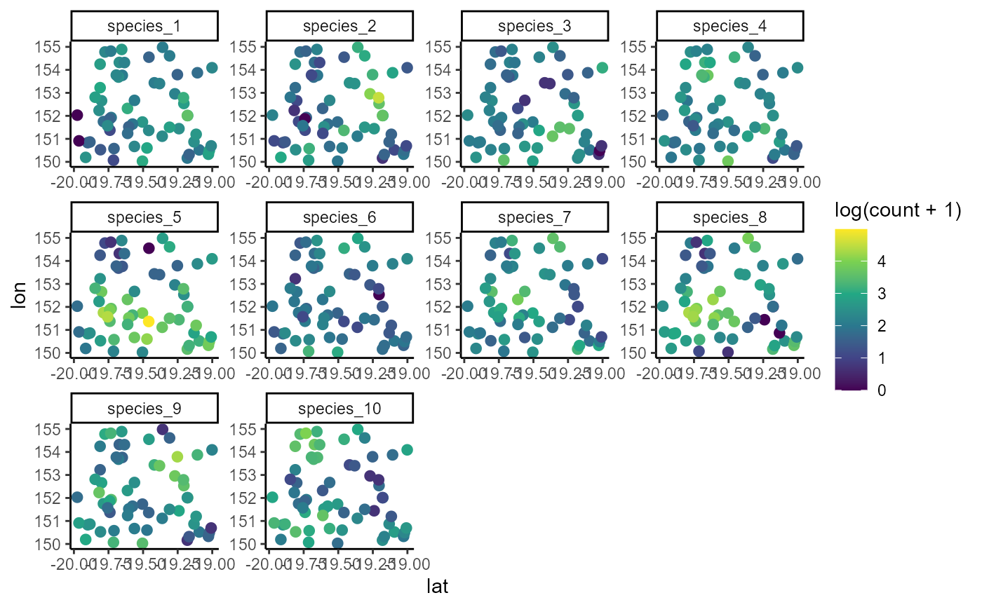
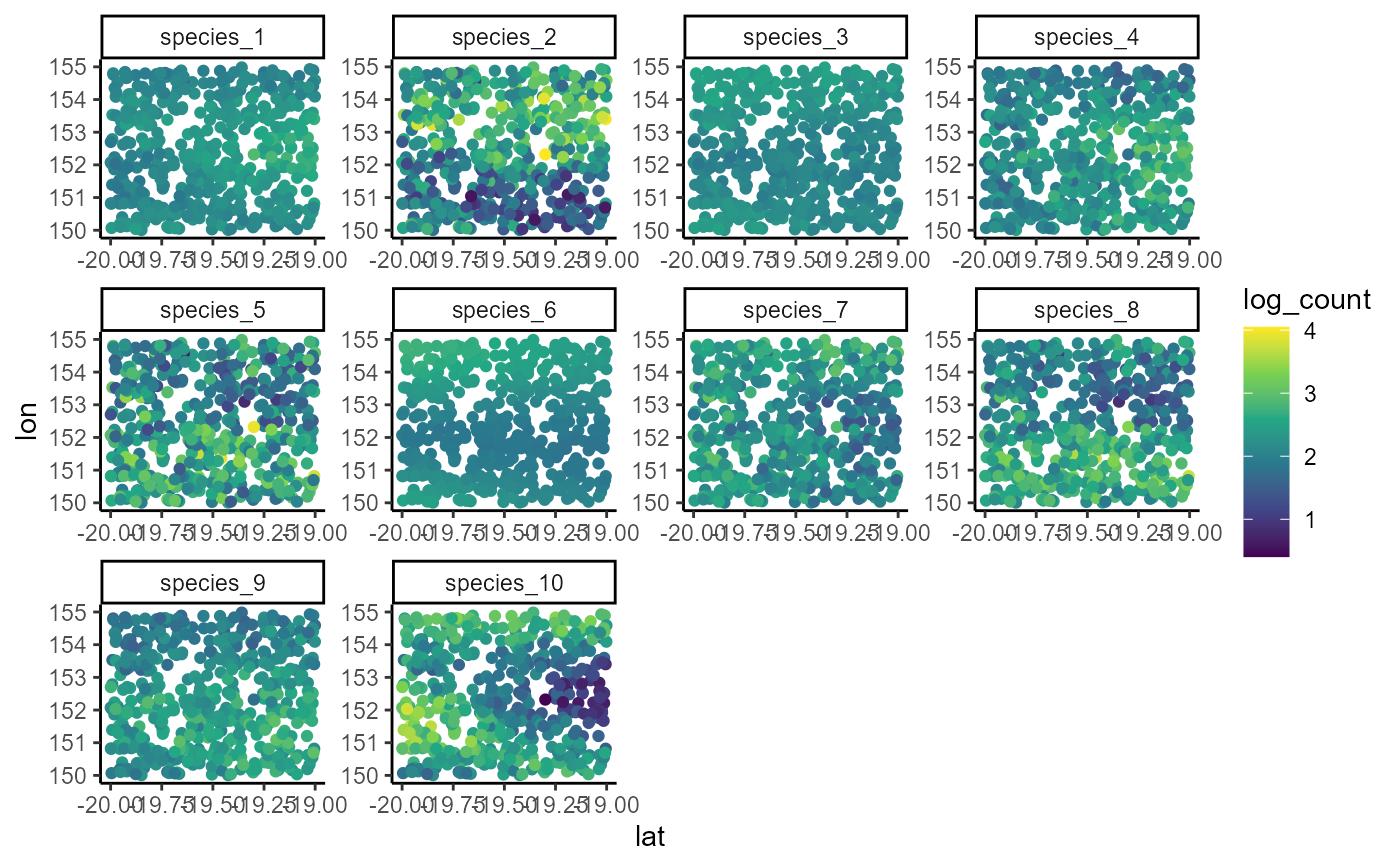
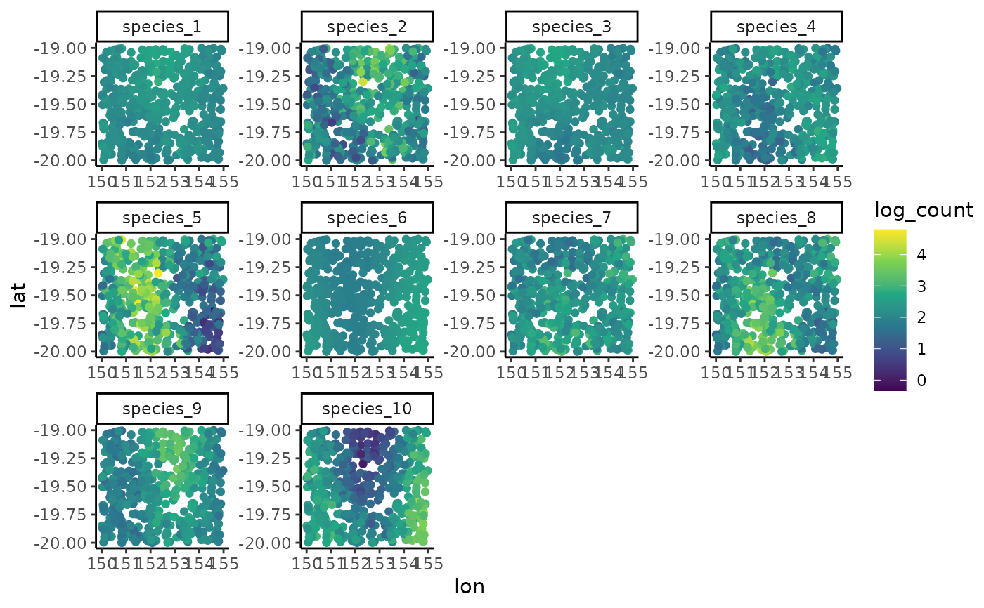
 ggplot(dat, aes(x = lon, y = lat, col = log(count + 1))) +
geom_point(size = 2.25) +
facet_wrap(~ species, scales = 'free') +
scale_color_viridis_c()
ggplot(dat, aes(x = lon, y = lat, col = log(count + 1))) +
geom_point(size = 2.25) +
facet_wrap(~ species, scales = 'free') +
scale_color_viridis_c()
 # ------------------------------------------------------------------------
# Model Fitting with Custom Priors
# ------------------------------------------------------------------------
# Inspect default priors for a joint species model with three spatial factors
priors <- get_mvgam_priors(
formula = count ~
# Environmental model includes random slopes for
# a linear effect of temperature
s(species, bs = 're', by = temperature),
# Each factor estimates a different nonlinear spatial process, using
# 'by = trend' as in other mvgam State-Space models
factor_formula = ~ gp(lon, lat, k = 6, by = trend) - 1,
n_lv = 3,
# The data and grouping variables
data = dat,
unit = site,
species = species,
# Poisson observations
family = poisson()
)
head(priors)
#> param_name param_length
#> 1 (Intercept) 1
#> 2 vector[1] mu_raw; 1
#> 3 vector<lower=0>[1] sigma_raw; 1
#> 4 real<lower=0> alpha_gp_trend(lon, lat):trendtrend1; 1
#> 5 real<lower=0> alpha_gp_trend(lon, lat):trendtrend2; 1
#> 6 real<lower=0> alpha_gp_trend(lon, lat):trendtrend3; 1
#> param_info
#> 1 (Intercept)
#> 2 s(species):temperature pop mean
#> 3 s(species):temperature pop sd
#> 4 gp(lon, lat):trendtrend1 marginal deviation
#> 5 gp(lon, lat):trendtrend2 marginal deviation
#> 6 gp(lon, lat):trendtrend3 marginal deviation
#> prior
#> 1 (Intercept) ~ student_t(3, 2.1, 2.5);
#> 2 mu_raw ~ std_normal();
#> 3 sigma_raw ~ inv_gamma(1.418, 0.452);
#> 4 alpha_gp_trend(lon, lat):trendtrend1 ~ student_t(3, 0, 2.5);
#> 5 alpha_gp_trend(lon, lat):trendtrend2 ~ student_t(3, 0, 2.5);
#> 6 alpha_gp_trend(lon, lat):trendtrend3 ~ student_t(3, 0, 2.5);
#> example_change new_lowerbound
#> 1 (Intercept) ~ normal(0, 1); <NA>
#> 2 mu_raw ~ normal(0.65, 0.15); <NA>
#> 3 sigma_raw ~ exponential(0.27); <NA>
#> 4 alpha_gp_trend(lon, lat):trendtrend1 ~ normal(0, 0.86); <NA>
#> 5 alpha_gp_trend(lon, lat):trendtrend2 ~ normal(0, 0.84); <NA>
#> 6 alpha_gp_trend(lon, lat):trendtrend3 ~ normal(0, 0.78); <NA>
#> new_upperbound
#> 1 <NA>
#> 2 <NA>
#> 3 <NA>
#> 4 <NA>
#> 5 <NA>
#> 6 <NA>
# Fit a JSDM that estimates hierarchical temperature responses
# and that uses three latent spatial factors
mod <- jsdgam(
formula = count ~
# Environmental model includes random slopes for a
# linear effect of temperature
s(species, bs = 're', by = temperature),
# Each factor estimates a different nonlinear spatial process, using
# 'by = trend' as in other mvgam State-Space models
factor_formula = ~ gp(lon, lat, k = 6, by = trend) - 1,
n_lv = 3,
# Change default priors for fixed random effect variances and
# factor GP marginal deviations to standard normal
priors = c(
prior(std_normal(), class = sigma_raw),
prior(std_normal(), class = `alpha_gp_trend(lon, lat):trendtrend1`),
prior(std_normal(), class = `alpha_gp_trend(lon, lat):trendtrend2`),
prior(std_normal(), class = `alpha_gp_trend(lon, lat):trendtrend3`)
),
# The data and the grouping variables
data = dat,
unit = site,
species = species,
# Poisson observations
family = poisson(),
chains = 2,
silent = 2
)
# ------------------------------------------------------------------------
# Model Visualization and Diagnostics
# ------------------------------------------------------------------------
# Plot the implicit species-level intercept estimates
plot_predictions(mod, condition = 'species', type = 'link')
# ------------------------------------------------------------------------
# Model Fitting with Custom Priors
# ------------------------------------------------------------------------
# Inspect default priors for a joint species model with three spatial factors
priors <- get_mvgam_priors(
formula = count ~
# Environmental model includes random slopes for
# a linear effect of temperature
s(species, bs = 're', by = temperature),
# Each factor estimates a different nonlinear spatial process, using
# 'by = trend' as in other mvgam State-Space models
factor_formula = ~ gp(lon, lat, k = 6, by = trend) - 1,
n_lv = 3,
# The data and grouping variables
data = dat,
unit = site,
species = species,
# Poisson observations
family = poisson()
)
head(priors)
#> param_name param_length
#> 1 (Intercept) 1
#> 2 vector[1] mu_raw; 1
#> 3 vector<lower=0>[1] sigma_raw; 1
#> 4 real<lower=0> alpha_gp_trend(lon, lat):trendtrend1; 1
#> 5 real<lower=0> alpha_gp_trend(lon, lat):trendtrend2; 1
#> 6 real<lower=0> alpha_gp_trend(lon, lat):trendtrend3; 1
#> param_info
#> 1 (Intercept)
#> 2 s(species):temperature pop mean
#> 3 s(species):temperature pop sd
#> 4 gp(lon, lat):trendtrend1 marginal deviation
#> 5 gp(lon, lat):trendtrend2 marginal deviation
#> 6 gp(lon, lat):trendtrend3 marginal deviation
#> prior
#> 1 (Intercept) ~ student_t(3, 2.1, 2.5);
#> 2 mu_raw ~ std_normal();
#> 3 sigma_raw ~ inv_gamma(1.418, 0.452);
#> 4 alpha_gp_trend(lon, lat):trendtrend1 ~ student_t(3, 0, 2.5);
#> 5 alpha_gp_trend(lon, lat):trendtrend2 ~ student_t(3, 0, 2.5);
#> 6 alpha_gp_trend(lon, lat):trendtrend3 ~ student_t(3, 0, 2.5);
#> example_change new_lowerbound
#> 1 (Intercept) ~ normal(0, 1); <NA>
#> 2 mu_raw ~ normal(0.65, 0.15); <NA>
#> 3 sigma_raw ~ exponential(0.27); <NA>
#> 4 alpha_gp_trend(lon, lat):trendtrend1 ~ normal(0, 0.86); <NA>
#> 5 alpha_gp_trend(lon, lat):trendtrend2 ~ normal(0, 0.84); <NA>
#> 6 alpha_gp_trend(lon, lat):trendtrend3 ~ normal(0, 0.78); <NA>
#> new_upperbound
#> 1 <NA>
#> 2 <NA>
#> 3 <NA>
#> 4 <NA>
#> 5 <NA>
#> 6 <NA>
# Fit a JSDM that estimates hierarchical temperature responses
# and that uses three latent spatial factors
mod <- jsdgam(
formula = count ~
# Environmental model includes random slopes for a
# linear effect of temperature
s(species, bs = 're', by = temperature),
# Each factor estimates a different nonlinear spatial process, using
# 'by = trend' as in other mvgam State-Space models
factor_formula = ~ gp(lon, lat, k = 6, by = trend) - 1,
n_lv = 3,
# Change default priors for fixed random effect variances and
# factor GP marginal deviations to standard normal
priors = c(
prior(std_normal(), class = sigma_raw),
prior(std_normal(), class = `alpha_gp_trend(lon, lat):trendtrend1`),
prior(std_normal(), class = `alpha_gp_trend(lon, lat):trendtrend2`),
prior(std_normal(), class = `alpha_gp_trend(lon, lat):trendtrend3`)
),
# The data and the grouping variables
data = dat,
unit = site,
species = species,
# Poisson observations
family = poisson(),
chains = 2,
silent = 2
)
# ------------------------------------------------------------------------
# Model Visualization and Diagnostics
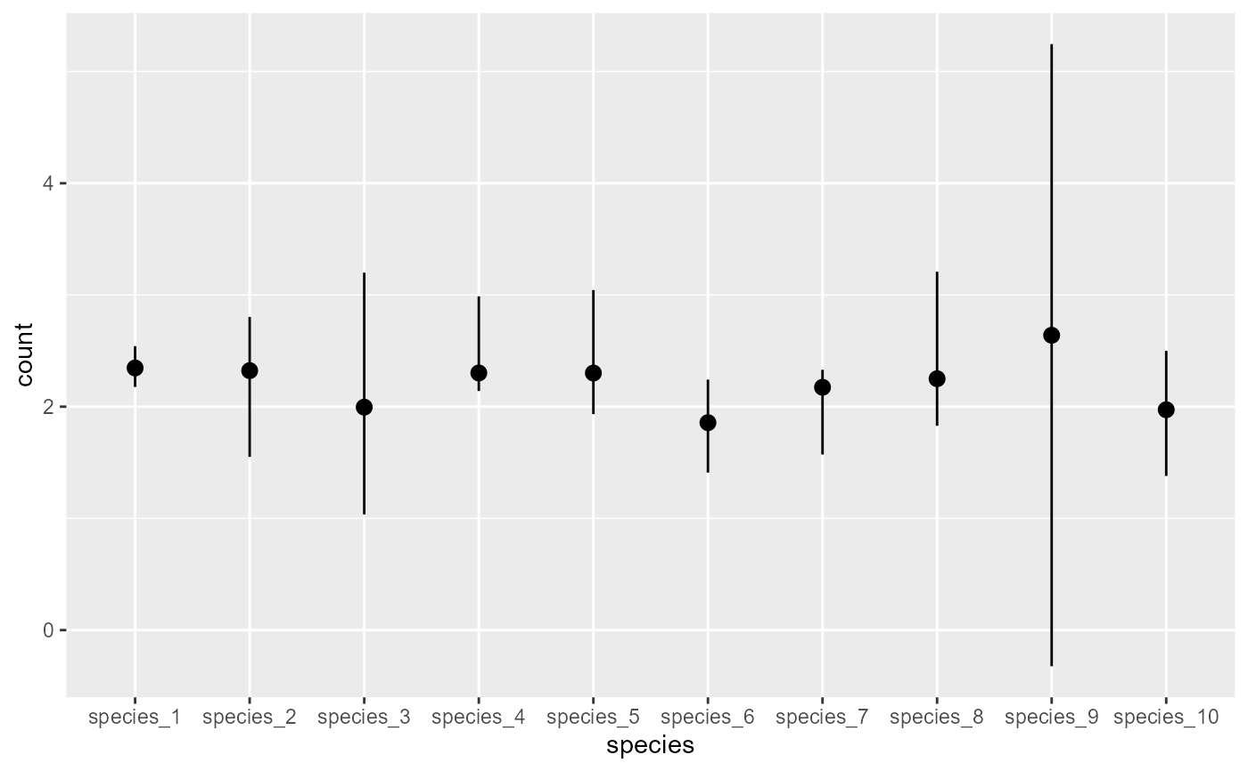
# ------------------------------------------------------------------------
# Plot the implicit species-level intercept estimates
plot_predictions(mod, condition = 'species', type = 'link')
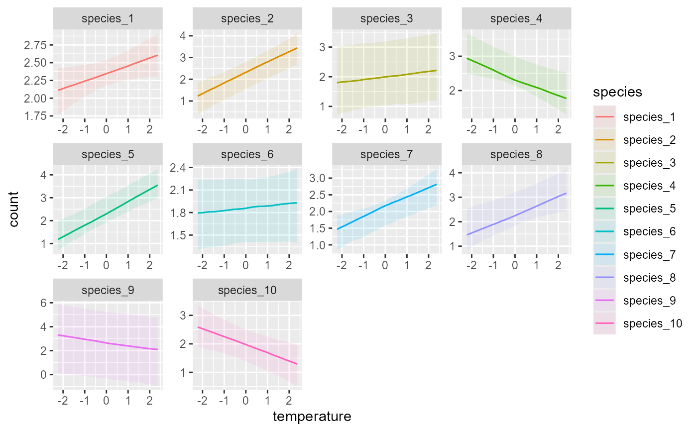
 # Plot species' hierarchical responses to temperature
plot_predictions(
mod,
condition = c('temperature', 'species', 'species'),
type = 'link'
)
# Plot species' hierarchical responses to temperature
plot_predictions(
mod,
condition = c('temperature', 'species', 'species'),
type = 'link'
)
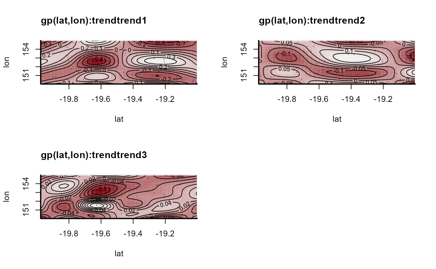
 # Plot posterior median estimates of the latent spatial factors
plot(mod, type = 'smooths', trend_effects = TRUE)
# Plot posterior median estimates of the latent spatial factors
plot(mod, type = 'smooths', trend_effects = TRUE)
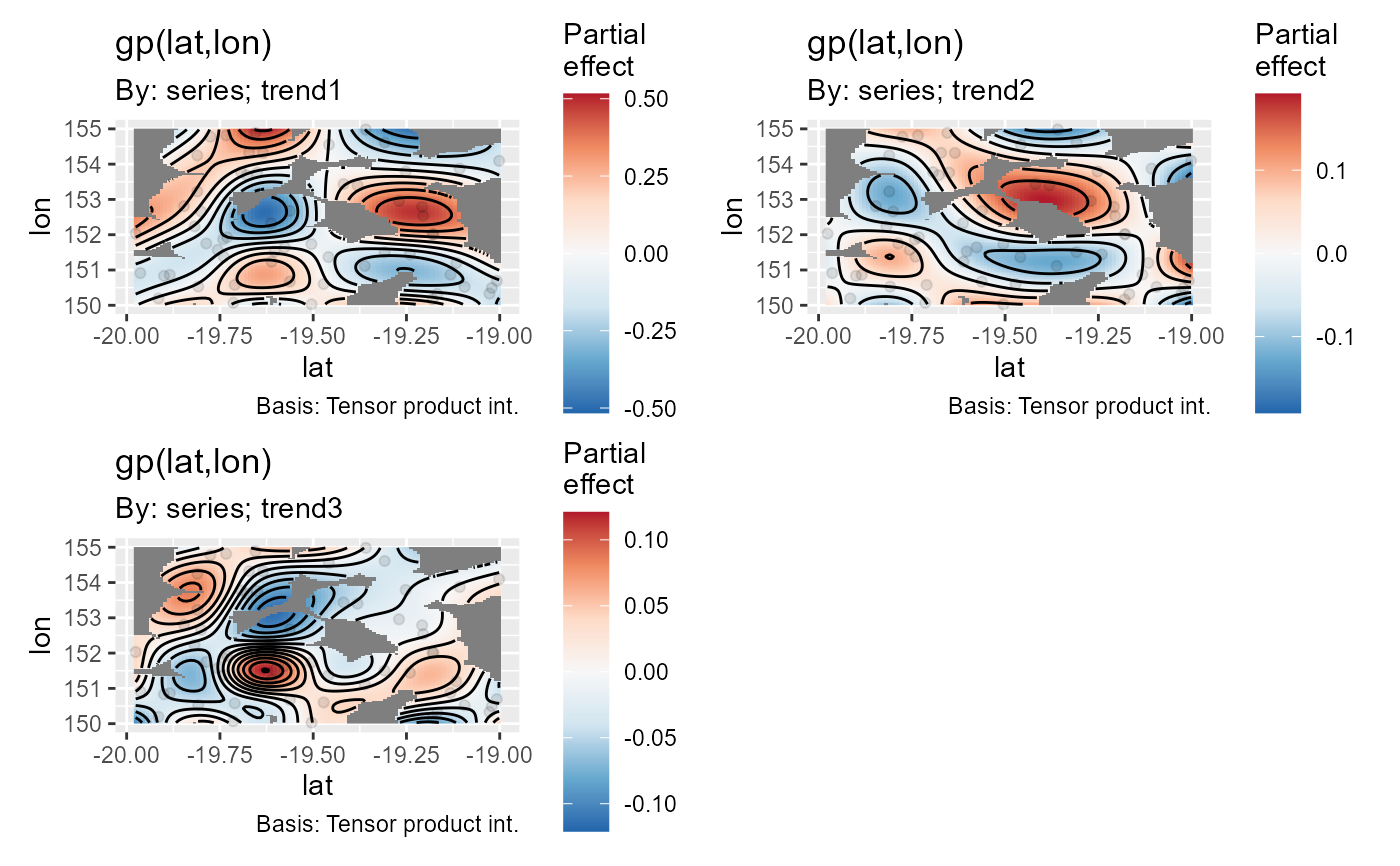
 # Or using gratia, if you have it installed
if(requireNamespace('gratia', quietly = TRUE)){
gratia::draw(mod, trend_effects = TRUE, dist = 0)
}
# Or using gratia, if you have it installed
if(requireNamespace('gratia', quietly = TRUE)){
gratia::draw(mod, trend_effects = TRUE, dist = 0)
}
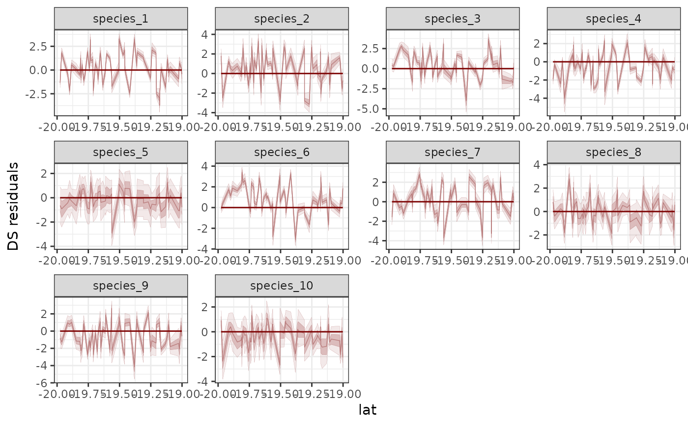
 # Plot species' randomized quantile residual distributions
# as a function of latitude
pp_check(
mod,
type = 'resid_ribbon_grouped',
group = 'species',
x = 'lat',
ndraws = 200
)
# Plot species' randomized quantile residual distributions
# as a function of latitude
pp_check(
mod,
type = 'resid_ribbon_grouped',
group = 'species',
x = 'lat',
ndraws = 200
)
 # ------------------------------------------------------------------------
# Residual Correlation Analysis
# ------------------------------------------------------------------------
# Calculate residual spatial correlations
post_cors <- residual_cor(mod)
names(post_cors)
#> [1] "cor" "cor_lower" "cor_upper" "sig_cor" "cov"
#> [6] "prec" "prec_lower" "prec_upper" "sig_prec" "trace"
# Look at lower and upper credible interval estimates for
# some of the estimated correlations
post_cors$cor[1:5, 1:5]
#> species_1 species_2 species_3 species_4 species_5
#> species_1 1.0000000 0.7478131 0.7077590 0.7584940 -0.2226666
#> species_2 0.7478131 1.0000000 0.1847152 0.4121104 -0.4646831
#> species_3 0.7077590 0.1847152 1.0000000 0.8893192 -0.0605947
#> species_4 0.7584940 0.4121104 0.8893192 1.0000000 -0.4702592
#> species_5 -0.2226666 -0.4646831 -0.0605947 -0.4702592 1.0000000
post_cors$cor_upper[1:5, 1:5]
#> species_1 species_2 species_3 species_4 species_5
#> species_1 1.0000000 0.9490107 0.9502659 0.9530001 0.2554003
#> species_2 0.9490107 1.0000000 0.5245854 0.7150460 -0.1225553
#> species_3 0.9502659 0.5245854 1.0000000 0.9724251 0.3063927
#> species_4 0.9530001 0.7150460 0.9724251 1.0000000 -0.1192866
#> species_5 0.2554003 -0.1225553 0.3063927 -0.1192866 1.0000000
post_cors$cor_lower[1:5, 1:5]
#> species_1 species_2 species_3 species_4 species_5
#> species_1 1.0000000 0.43039541 0.2587199 0.27620555 -0.5832631
#> species_2 0.4303954 1.00000000 -0.2033173 0.01403026 -0.7246616
#> species_3 0.2587199 -0.20331727 1.0000000 0.73412062 -0.4171413
#> species_4 0.2762055 0.01403026 0.7341206 1.00000000 -0.7275829
#> species_5 -0.5832631 -0.72466157 -0.4171413 -0.72758293 1.0000000
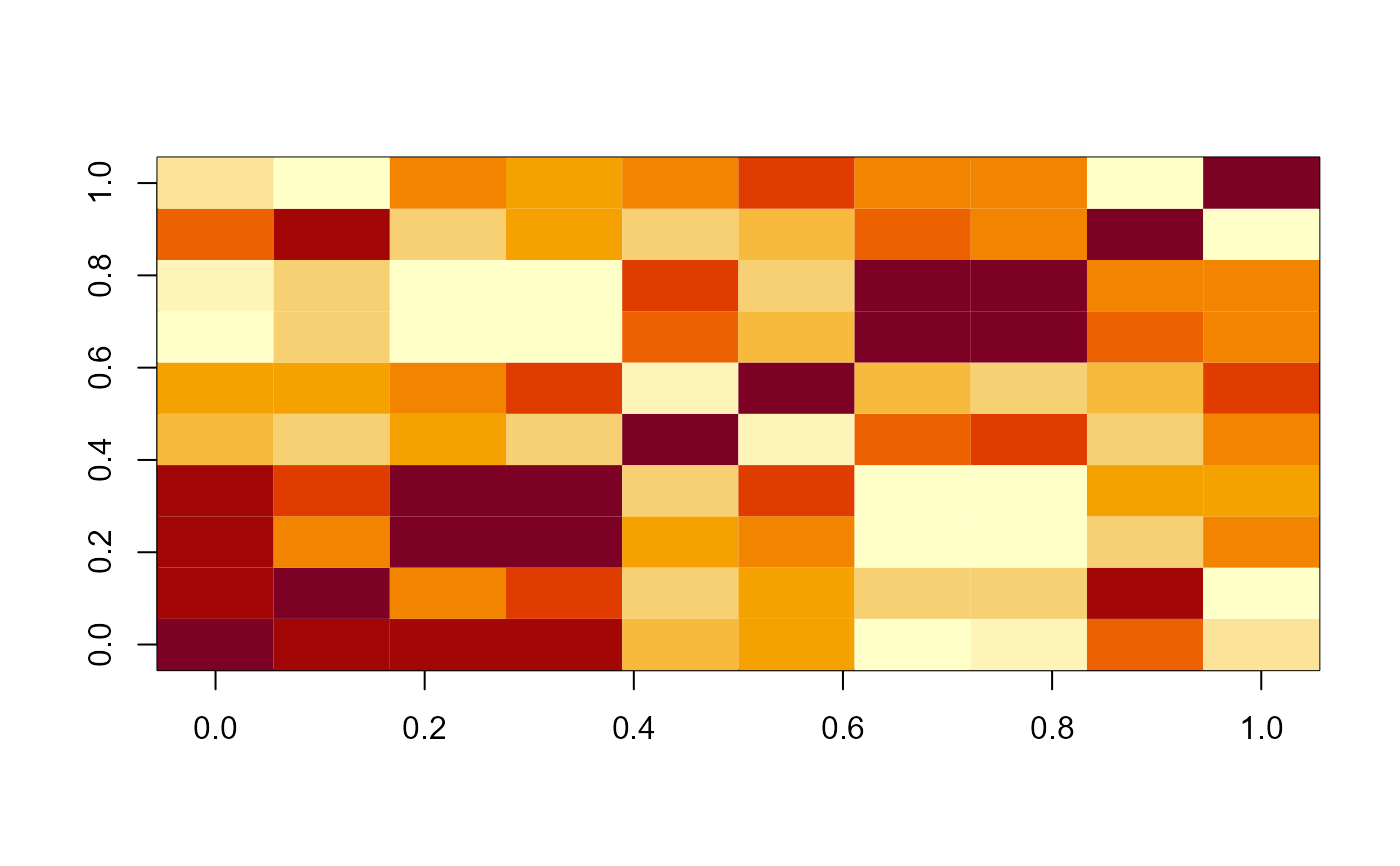
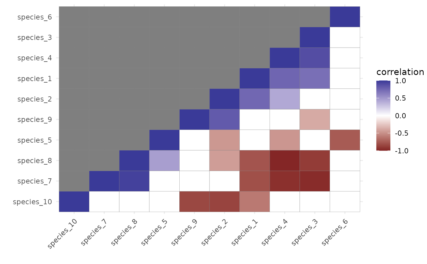
# Plot of the posterior median correlations for those estimated
# to be non-zero
plot(post_cors, cluster = TRUE)
# ------------------------------------------------------------------------
# Residual Correlation Analysis
# ------------------------------------------------------------------------
# Calculate residual spatial correlations
post_cors <- residual_cor(mod)
names(post_cors)
#> [1] "cor" "cor_lower" "cor_upper" "sig_cor" "cov"
#> [6] "prec" "prec_lower" "prec_upper" "sig_prec" "trace"
# Look at lower and upper credible interval estimates for
# some of the estimated correlations
post_cors$cor[1:5, 1:5]
#> species_1 species_2 species_3 species_4 species_5
#> species_1 1.0000000 0.7478131 0.7077590 0.7584940 -0.2226666
#> species_2 0.7478131 1.0000000 0.1847152 0.4121104 -0.4646831
#> species_3 0.7077590 0.1847152 1.0000000 0.8893192 -0.0605947
#> species_4 0.7584940 0.4121104 0.8893192 1.0000000 -0.4702592
#> species_5 -0.2226666 -0.4646831 -0.0605947 -0.4702592 1.0000000
post_cors$cor_upper[1:5, 1:5]
#> species_1 species_2 species_3 species_4 species_5
#> species_1 1.0000000 0.9490107 0.9502659 0.9530001 0.2554003
#> species_2 0.9490107 1.0000000 0.5245854 0.7150460 -0.1225553
#> species_3 0.9502659 0.5245854 1.0000000 0.9724251 0.3063927
#> species_4 0.9530001 0.7150460 0.9724251 1.0000000 -0.1192866
#> species_5 0.2554003 -0.1225553 0.3063927 -0.1192866 1.0000000
post_cors$cor_lower[1:5, 1:5]
#> species_1 species_2 species_3 species_4 species_5
#> species_1 1.0000000 0.43039541 0.2587199 0.27620555 -0.5832631
#> species_2 0.4303954 1.00000000 -0.2033173 0.01403026 -0.7246616
#> species_3 0.2587199 -0.20331727 1.0000000 0.73412062 -0.4171413
#> species_4 0.2762055 0.01403026 0.7341206 1.00000000 -0.7275829
#> species_5 -0.5832631 -0.72466157 -0.4171413 -0.72758293 1.0000000
# Plot of the posterior median correlations for those estimated
# to be non-zero
plot(post_cors, cluster = TRUE)
 # An ordination biplot can also be constructed
# from the factor scores and their loadings
if(requireNamespace('ggrepel', quietly = TRUE)){
ordinate(mod)
}
# An ordination biplot can also be constructed
# from the factor scores and their loadings
if(requireNamespace('ggrepel', quietly = TRUE)){
ordinate(mod)
}
 # ------------------------------------------------------------------------
# Model Validation and Prediction
# ------------------------------------------------------------------------
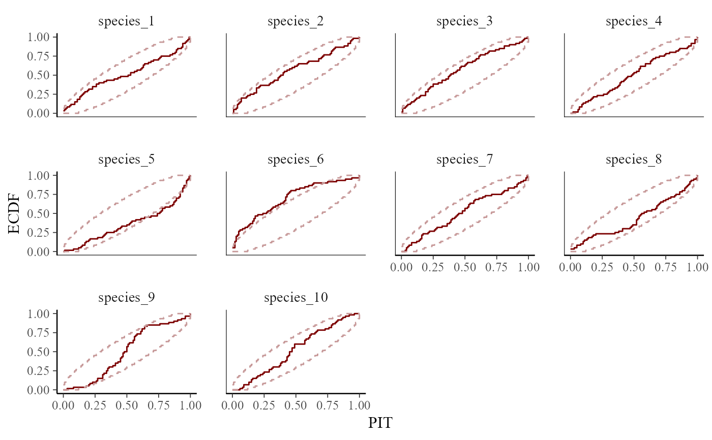
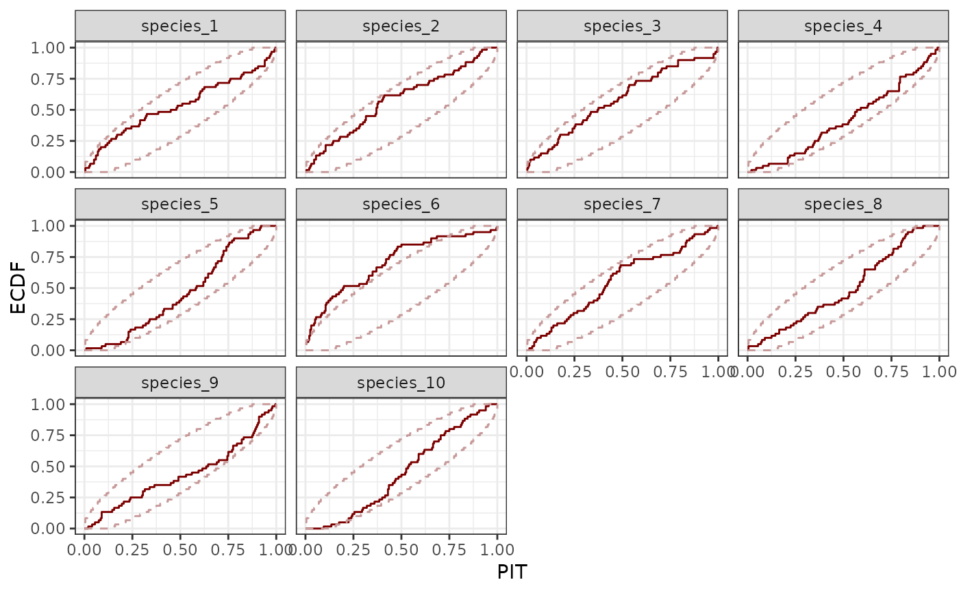
# Posterior predictive checks and ELPD-LOO can ascertain model fit
pp_check(
mod,
type = "pit_ecdf_grouped",
group = "species",
ndraws = 200
)
# ------------------------------------------------------------------------
# Model Validation and Prediction
# ------------------------------------------------------------------------
# Posterior predictive checks and ELPD-LOO can ascertain model fit
pp_check(
mod,
type = "pit_ecdf_grouped",
group = "species",
ndraws = 200
)
 loo(mod)
#> Warning: Some Pareto k diagnostic values are too high. See help('pareto-k-diagnostic') for details.
#>
#> Computed from 1000 by 600 log-likelihood matrix.
#>
#> Estimate SE
#> elpd_loo -4465.3 231.5
#> p_loo 2266.2 191.4
#> looic 8930.6 463.1
#> ------
#> MCSE of elpd_loo is NA.
#> MCSE and ESS estimates assume MCMC draws (r_eff in [0.0, 1.1]).
#>
#> Pareto k diagnostic values:
#> Count Pct. Min. ESS
#> (-Inf, 0.67] (good) 319 53.2% 2
#> (0.67, 1] (bad) 94 15.7% <NA>
#> (1, Inf) (very bad) 187 31.2% <NA>
#> See help('pareto-k-diagnostic') for details.
# Forecast log(counts) for entire region (site value doesn't matter as long
# as each spatial location has a different and unique site identifier);
# note this calculation takes a few minutes because of the need to calculate
# draws from the stochastic latent factors
newdata <- st_process %>%
dplyr::mutate(species = factor(
species,
levels = paste0('species_', 1:N_species)
)) %>%
dplyr::group_by(lat, lon) %>%
dplyr::mutate(site = dplyr::cur_group_id()) %>%
dplyr::ungroup()
preds <- predict(mod, newdata = newdata)
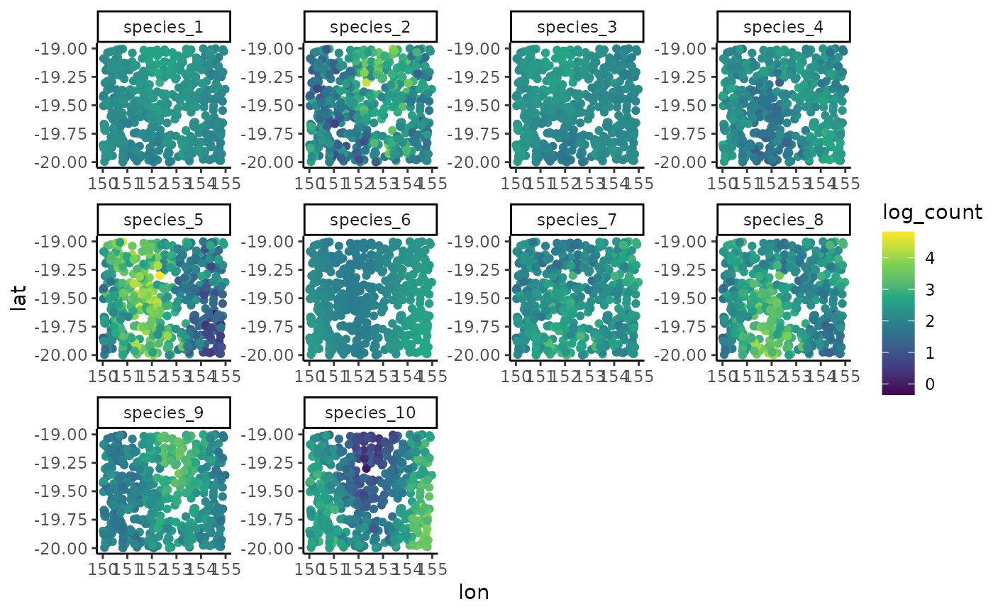
# Plot the median log(count) predictions on a grid
newdata$log_count <- preds[,1]
ggplot(newdata, aes(x = lon, y = lat, col = log_count)) +
geom_point(size = 1.5) +
facet_wrap(~ species, scales = 'free') +
scale_color_viridis_c() +
theme_classic()
loo(mod)
#> Warning: Some Pareto k diagnostic values are too high. See help('pareto-k-diagnostic') for details.
#>
#> Computed from 1000 by 600 log-likelihood matrix.
#>
#> Estimate SE
#> elpd_loo -4465.3 231.5
#> p_loo 2266.2 191.4
#> looic 8930.6 463.1
#> ------
#> MCSE of elpd_loo is NA.
#> MCSE and ESS estimates assume MCMC draws (r_eff in [0.0, 1.1]).
#>
#> Pareto k diagnostic values:
#> Count Pct. Min. ESS
#> (-Inf, 0.67] (good) 319 53.2% 2
#> (0.67, 1] (bad) 94 15.7% <NA>
#> (1, Inf) (very bad) 187 31.2% <NA>
#> See help('pareto-k-diagnostic') for details.
# Forecast log(counts) for entire region (site value doesn't matter as long
# as each spatial location has a different and unique site identifier);
# note this calculation takes a few minutes because of the need to calculate
# draws from the stochastic latent factors
newdata <- st_process %>%
dplyr::mutate(species = factor(
species,
levels = paste0('species_', 1:N_species)
)) %>%
dplyr::group_by(lat, lon) %>%
dplyr::mutate(site = dplyr::cur_group_id()) %>%
dplyr::ungroup()
preds <- predict(mod, newdata = newdata)
# Plot the median log(count) predictions on a grid
newdata$log_count <- preds[,1]
ggplot(newdata, aes(x = lon, y = lat, col = log_count)) +
geom_point(size = 1.5) +
facet_wrap(~ species, scales = 'free') +
scale_color_viridis_c() +
theme_classic()
 # Not needed for general use; cleans up connections for automated testing
closeAllConnections()
# }
# Not needed for general use; cleans up connections for automated testing
closeAllConnections()
# }