Compute Generalized or Orthogonalized Impulse Response Functions (IRFs) from
mvgam models with Vector Autoregressive dynamics
Usage
irf(object, ...)

# S3 method for mvgam
irf(object, h = 10, cumulative = FALSE, orthogonal = FALSE, ...)
Arguments
- object
listobject of classmvgamresulting from a call tomvgam()that used a Vector Autoregressive latent process model (either asVAR(cor = FALSE)orVAR(cor = TRUE); seeVAR()for details)- ...
ignored
- h
Positive
integerspecifying the forecast horizon over which to calculate the IRF- cumulative
Logicalflag indicating whether the IRF should be cumulative- orthogonal
Logicalflag indicating whether orthogonalized IRFs should be calculated. Note that the order of the variables matters when calculating these
Value
An object of mvgam_irf-class containing the posterior IRFs. This
object can be used with the supplied S3 functions plot.mvgam_irf()
Details
See mvgam_irf-class for a full description of the quantities that are
computed and returned by this function, along with key references.
Examples
# \dontrun{
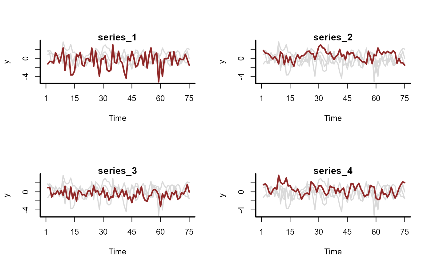
# Fit a model to the portal time series that uses a latent VAR(1)
mod <- mvgam(
formula = captures ~ -1,
trend_formula = ~ trend,
trend_model = VAR(cor = TRUE),
family = poisson(),
data = portal_data,
chains = 2,
silent = 2
)
# Plot the autoregressive coefficient distributions;
# use 'dir = "v"' to arrange the order of facets
# correctly
mcmc_plot(
mod,
variable = 'A',
regex = TRUE,
type = 'hist',
facet_args = list(dir = 'v')
)
#> `stat_bin()` using `bins = 30`. Pick better value `binwidth`.
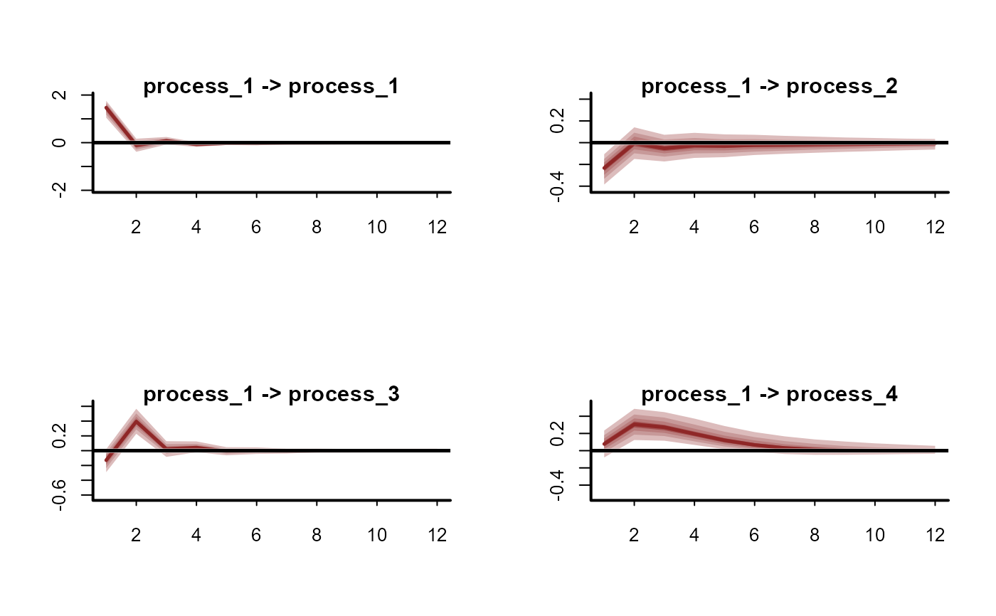
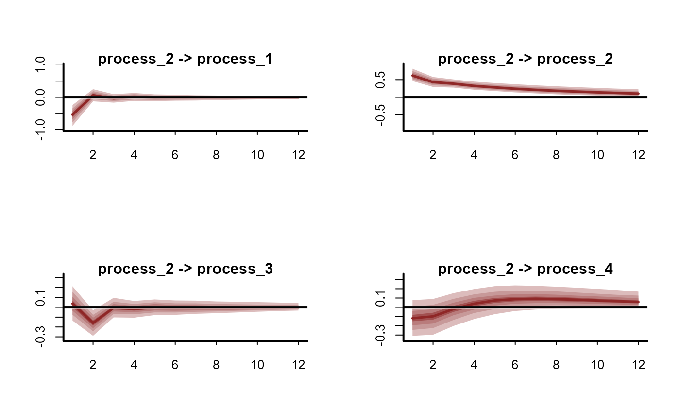
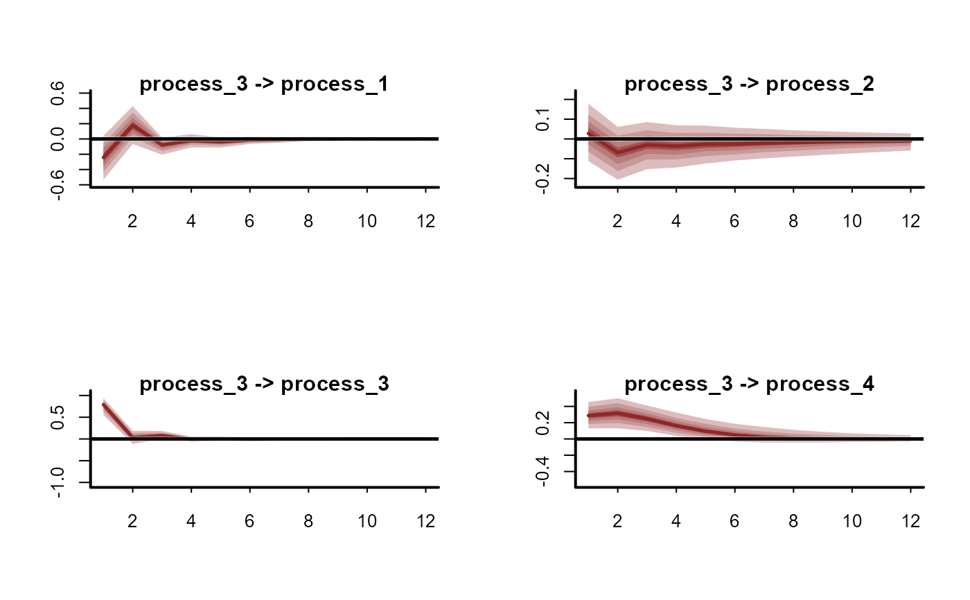
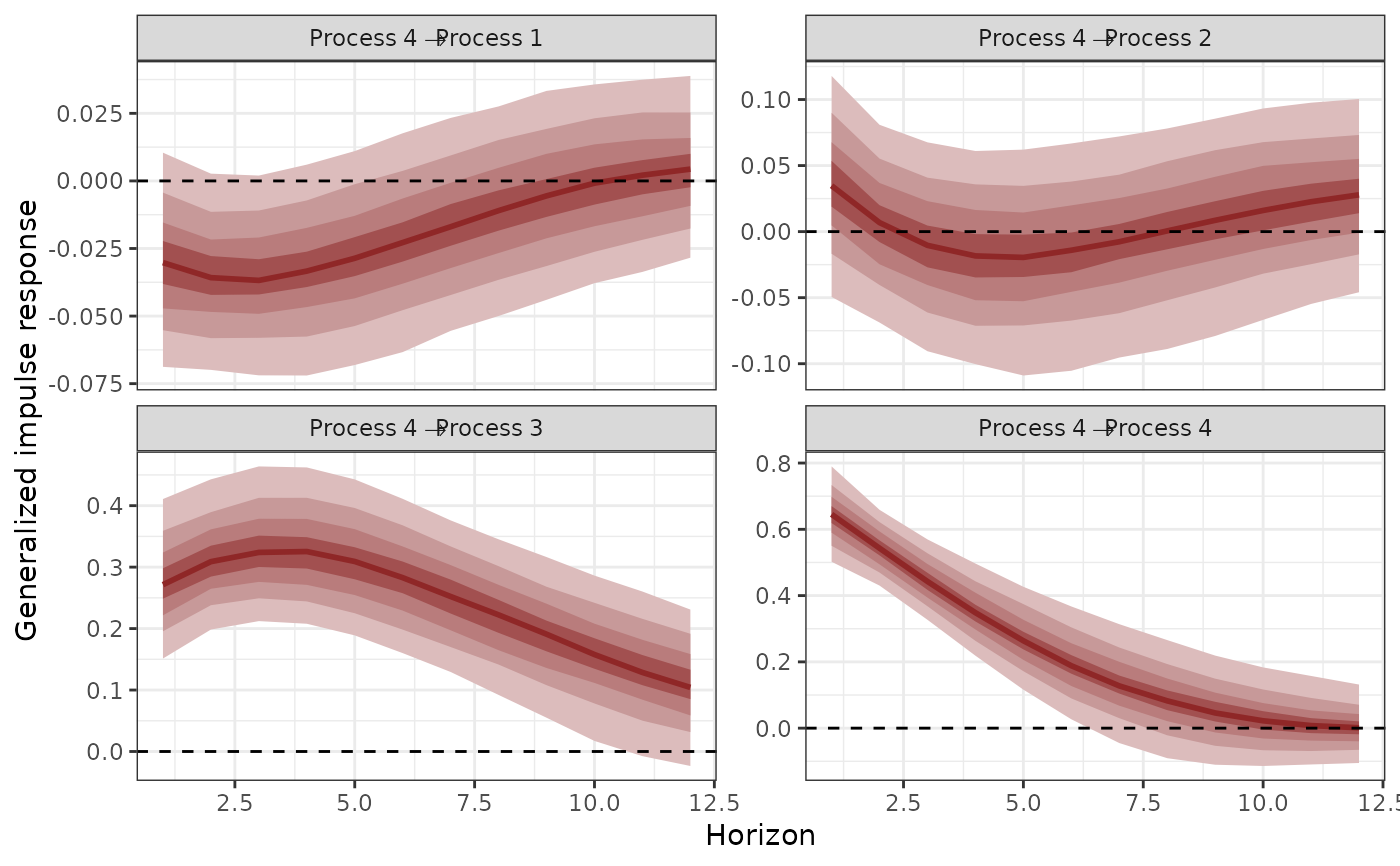
 # Calulate Generalized IRFs for each series
irfs <- irf(
mod,
h = 12,
cumulative = FALSE
)
# Plot them
plot(irfs, series = 1)
# Calulate Generalized IRFs for each series
irfs <- irf(
mod,
h = 12,
cumulative = FALSE
)
# Plot them
plot(irfs, series = 1)
 plot(irfs, series = 2)
 plot(irfs, series = 3)
 plot(irfs, series = 4)
 # Calculate posterior median, upper and lower 95th quantiles
# of the impulse responses
summary(irfs)
#> # A tibble: 192 × 5
#> shock horizon irfQ50 irfQ2.5 irfQ97.5
#> <chr> <int> <dbl> <dbl> <dbl>
#> 1 Process_1 -> Process_1 1 0.143 0.0886 0.221
#> 2 Process_1 -> Process_1 2 0.131 0.0829 0.197
#> 3 Process_1 -> Process_1 3 0.119 0.0731 0.182
#> 4 Process_1 -> Process_1 4 0.106 0.0624 0.170
#> 5 Process_1 -> Process_1 5 0.0940 0.0486 0.158
#> 6 Process_1 -> Process_1 6 0.0835 0.0370 0.147
#> 7 Process_1 -> Process_1 7 0.0739 0.0258 0.139
#> 8 Process_1 -> Process_1 8 0.0646 0.0160 0.135
#> 9 Process_1 -> Process_1 9 0.0567 0.00877 0.129
#> 10 Process_1 -> Process_1 10 0.0494 0.000988 0.124
#> # ℹ 182 more rows
# }
# Calculate posterior median, upper and lower 95th quantiles
# of the impulse responses
summary(irfs)
#> # A tibble: 192 × 5
#> shock horizon irfQ50 irfQ2.5 irfQ97.5
#> <chr> <int> <dbl> <dbl> <dbl>
#> 1 Process_1 -> Process_1 1 0.143 0.0886 0.221
#> 2 Process_1 -> Process_1 2 0.131 0.0829 0.197
#> 3 Process_1 -> Process_1 3 0.119 0.0731 0.182
#> 4 Process_1 -> Process_1 4 0.106 0.0624 0.170
#> 5 Process_1 -> Process_1 5 0.0940 0.0486 0.158
#> 6 Process_1 -> Process_1 6 0.0835 0.0370 0.147
#> 7 Process_1 -> Process_1 7 0.0739 0.0258 0.139
#> 8 Process_1 -> Process_1 8 0.0646 0.0160 0.135
#> 9 Process_1 -> Process_1 9 0.0567 0.00877 0.129
#> 10 Process_1 -> Process_1 10 0.0494 0.000988 0.124
#> # ℹ 182 more rows
# }