Specify piecewise linear or logistic trends in mvgam models
Source:R/mvgam_trend_types.R
piecewise_trends.RdSet up piecewise linear or logistic trend models in mvgam. These
functions do not evaluate their arguments – they exist purely to help set up
a model with particular piecewise trend models.
Usage
PW(
  n_changepoints = 10,
  changepoint_range = 0.8,
  changepoint_scale = 0.05,
  growth = "linear"
)
Arguments
- n_changepoints
A non-negative integer specifying the number of potential changepoints. Potential changepoints are selected uniformly from the first
changepoint_rangeproportion of timepoints indata. Default is10.- changepoint_range
Proportion of history in
datain which trend changepoints will be estimated. Defaults to0.8for the first 80%.- changepoint_scale
Parameter modulating the flexibility of the automatic changepoint selection by altering the scale parameter of a Laplace distribution. The resulting prior will be
double_exponential(0, changepoint_scale). Large values will allow many changepoints and a more flexible trend, while small values will allow few changepoints. Default is0.05.- growth
Character string specifying either
'linear'or'logistic'growth of the trend. If'logistic', a variable labelledcapMUST be indatato specify the maximum saturation point for the trend (see details and examples inmvgamfor more information). Default is'linear'.
Value
An object of class mvgam_trend, which contains a list of
arguments to be interpreted by the parsing functions in mvgam.
Details
Offsets and intercepts:
For each of these trend models, an offset parameter is included in the trend
estimation process. This parameter will be incredibly difficult to identify
if you also include an intercept in the observation formula. For that
reason, it is highly recommended that you drop the intercept from the
formula (i.e. y ~ x + 0 or y ~ x - 1, where x are your optional
predictor terms).
Logistic growth and the cap variable: When forecasting growth, there is often some maximum achievable point that a time series can reach. For example, total market size, total population size or carrying capacity in population dynamics. It can be advantageous for the forecast to saturate at or near this point so that predictions are more sensible.
This function allows you to make forecasts using a logistic growth trend
model, with a specified carrying capacity. Note that this capacity does not
need to be static over time; it can vary with each series × timepoint
combination if necessary. But you must supply a cap value for each
observation in the data when using growth = 'logistic'.
For observation families that use a non-identity link function, the cap
value will be internally transformed to the link scale (i.e. your specified
cap will be log-transformed if you are using a poisson() or nb()
family). It is therefore important that you specify the cap values on the
scale of your outcome. Note also that no missing values are allowed in
cap.
References
Taylor, Sean J., and Benjamin Letham. "Forecasting at scale." The American Statistician 72.1 (2018): 37–45.
Examples
# \dontrun{
# Example of logistic growth with possible changepoints
dNt = function(r, N, k) {
r * N * (k - N)
}
Nt = function(r, N, t, k) {
for (i in 1:(t - 1)) {
if (i %in% c(5, 15, 25, 41, 45, 60, 80)) {
N[i + 1] <- max(
1,
N[i] + dNt(r + runif(1, -0.1, 0.1), N[i], k)
)
} else {
N[i + 1] <- max(1, N[i] + dNt(r, N[i], k))
}
}
N
}
set.seed(11)
expected <- Nt(0.004, 2, 100, 30)
plot(expected, xlab = 'Time')
 y <- rpois(100, expected)
plot(y, xlab = 'Time')
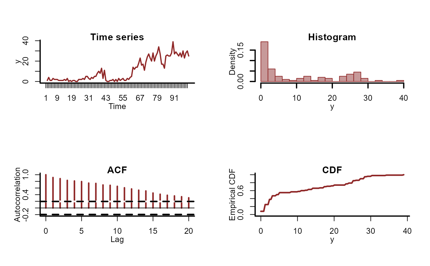
y <- rpois(100, expected)
plot(y, xlab = 'Time')
 mod_data <- data.frame(
y = y,
time = 1:100,
cap = 35,
series = as.factor('series_1')
)
plot_mvgam_series(data = mod_data)
mod_data <- data.frame(
y = y,
time = 1:100,
cap = 35,
series = as.factor('series_1')
)
plot_mvgam_series(data = mod_data)
 mod <- mvgam(
y ~ 0,
trend_model = PW(growth = 'logistic'),
family = poisson(),
data = mod_data,
chains = 2,
silent = 2
)
summary(mod)
#> GAM formula:
#> y ~ 1
#> <environment: 0x5582e9f95190>
#>
#> Family:
#> poisson
#>
#> Link function:
#> log
#>
#> Trend model:
#> PW(growth = "logistic")
#>
#> N series:
#> 1
#>
#> N timepoints:
#> 100
#>
#> Status:
#> Fitted using Stan
#> 2 chains, each with iter = 1000; warmup = 500; thin = 1
#> Total post-warmup draws = 1000
#>
#> GAM coefficient (beta) estimates:
#> 2.5% 50% 97.5% Rhat n_eff
#> (Intercept) 0 0 0 NaN NaN
#>
#> growth rate:
#> 2.5% 50% 97.5% Rhat n_eff
#> k_trend[1] -0.28 -0.15 -0.07 1 578
#>
#> offset parameter:
#> 2.5% 50% 97.5% Rhat n_eff
#> m_trend[1] -18 -4.2 -0.24 1 318
#>
#> Stan MCMC diagnostics:
#> ✔ No issues with effective samples per iteration
#> ✔ Rhat looks good for all parameters
#> ✔ No issues with divergences
#> ✖ 234 of 1000 iterations saturated the maximum tree depth of 10 (23.4%)
#> Try a larger max_treedepth to avoid saturation
#>
#> Samples were drawn using sampling(hmc). For each parameter, n_eff is a
#> crude measure of effective sample size, and Rhat is the potential scale
#> reduction factor on split MCMC chains (at convergence, Rhat = 1)
#>
#> Use how_to_cite() to get started describing this model
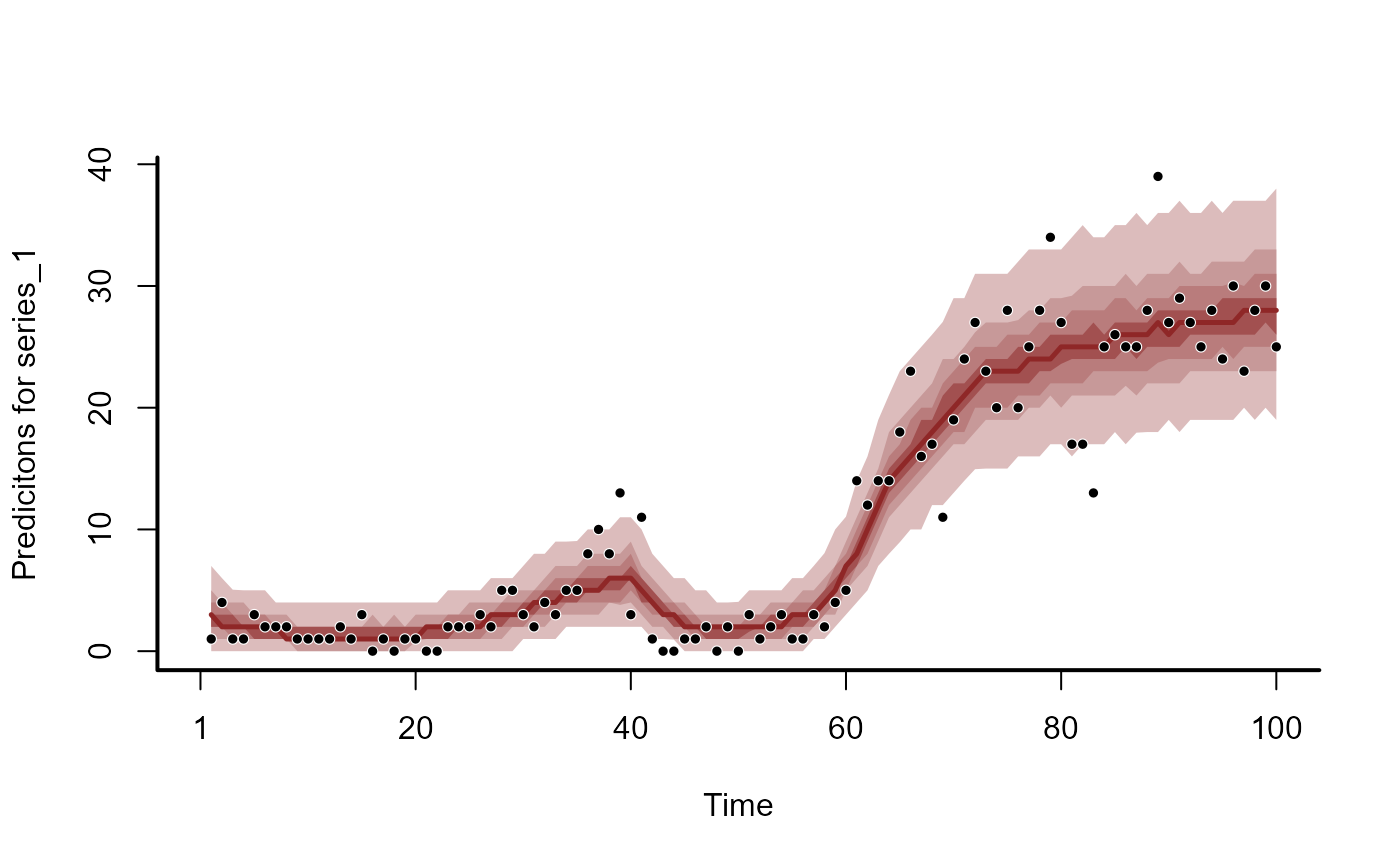
hc <- hindcast(mod)
plot(hc)
#> No non-missing values in test_observations; cannot calculate forecast score
mod <- mvgam(
y ~ 0,
trend_model = PW(growth = 'logistic'),
family = poisson(),
data = mod_data,
chains = 2,
silent = 2
)
summary(mod)
#> GAM formula:
#> y ~ 1
#> <environment: 0x5582e9f95190>
#>
#> Family:
#> poisson
#>
#> Link function:
#> log
#>
#> Trend model:
#> PW(growth = "logistic")
#>
#> N series:
#> 1
#>
#> N timepoints:
#> 100
#>
#> Status:
#> Fitted using Stan
#> 2 chains, each with iter = 1000; warmup = 500; thin = 1
#> Total post-warmup draws = 1000
#>
#> GAM coefficient (beta) estimates:
#> 2.5% 50% 97.5% Rhat n_eff
#> (Intercept) 0 0 0 NaN NaN
#>
#> growth rate:
#> 2.5% 50% 97.5% Rhat n_eff
#> k_trend[1] -0.28 -0.15 -0.07 1 578
#>
#> offset parameter:
#> 2.5% 50% 97.5% Rhat n_eff
#> m_trend[1] -18 -4.2 -0.24 1 318
#>
#> Stan MCMC diagnostics:
#> ✔ No issues with effective samples per iteration
#> ✔ Rhat looks good for all parameters
#> ✔ No issues with divergences
#> ✖ 234 of 1000 iterations saturated the maximum tree depth of 10 (23.4%)
#> Try a larger max_treedepth to avoid saturation
#>
#> Samples were drawn using sampling(hmc). For each parameter, n_eff is a
#> crude measure of effective sample size, and Rhat is the potential scale
#> reduction factor on split MCMC chains (at convergence, Rhat = 1)
#>
#> Use how_to_cite() to get started describing this model
hc <- hindcast(mod)
plot(hc)
#> No non-missing values in test_observations; cannot calculate forecast score
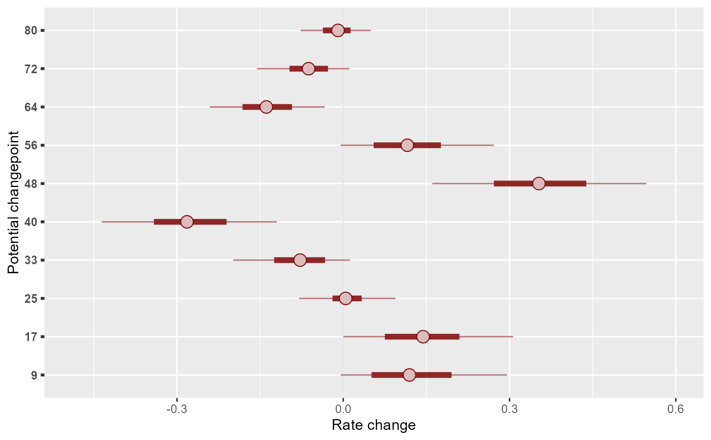
 library(ggplot2)
mcmc_plot(mod, variable = 'delta_trend', regex = TRUE) +
scale_y_discrete(labels = mod$trend_model$changepoints) +
labs(
y = 'Potential changepoint',
x = 'Rate change'
)
#> Scale for y is already present.
#> Adding another scale for y, which will replace the existing scale.
library(ggplot2)
mcmc_plot(mod, variable = 'delta_trend', regex = TRUE) +
scale_y_discrete(labels = mod$trend_model$changepoints) +
labs(
y = 'Potential changepoint',
x = 'Rate change'
)
#> Scale for y is already present.
#> Adding another scale for y, which will replace the existing scale.
 how_to_cite(mod)
#> Methods text skeleton
#> We used the R package mvgam (version 1.1.595; Clark & Wells, 2023) to
#> construct, fit and interrogate the model. mvgam fits Bayesian
#> State-Space models that can include flexible predictor effects in both
#> the process and observation components by incorporating functionalities
#> from the brms (Burkner 2017), mgcv (Wood 2017) and splines2 (Wang & Yan,
#> 2023) packages. Piecewise dynamic trends were parameterized and
#> estimated following methods described by Taylor and Letham (2018). The
#> mvgam-constructed model and observed data were passed to the
#> probabilistic programming environment Stan (version 2.38.0; Carpenter et
#> al. 2017, Stan Development Team 2026), specifically through the cmdstanr
#> interface (Gabry & Cesnovar, 2021). We ran 2 Hamiltonian Monte Carlo
#> chains for 500 warmup iterations and 500 sampling iterations for joint
#> posterior estimation. Rank normalized split Rhat (Vehtari et al. 2021)
#> and effective sample sizes were used to monitor convergence.
#>
#> Primary references
#> Clark, NJ and Wells K (2023). Dynamic Generalized Additive Models
#> (DGAMs) for forecasting discrete ecological time series. Methods in
#> Ecology and Evolution, 14, 771-784. doi.org/10.1111/2041-210X.13974
#> Burkner, PC (2017). brms: An R Package for Bayesian Multilevel Models
#> Using Stan. Journal of Statistical Software, 80(1), 1-28.
#> doi:10.18637/jss.v080.i01
#> Wood, SN (2017). Generalized Additive Models: An Introduction with R
#> (2nd edition). Chapman and Hall/CRC.
#> Wang W and Yan J (2021). Shape-Restricted Regression Splines with R
#> Package splines2. Journal of Data Science, 19(3), 498-517.
#> doi:10.6339/21-JDS1020 https://doi.org/10.6339/21-JDS1020.
#> Taylor S and Letham B (2018). Forecasting at scale. The American
#> Statistician 72(1) 37-45. https://doi.org/10.1080/00031305.2017.1380080
#> Carpenter B, Gelman A, Hoffman MD, Lee D, Goodrich B, Betancourt M,
#> Brubaker M, Guo J, Li P and Riddell A (2017). Stan: A probabilistic
#> programming language. Journal of Statistical Software 76.
#> Gabry J, Cesnovar R, Johnson A, and Bronder S (2026). cmdstanr: R
#> Interface to 'CmdStan'. https://mc-stan.org/cmdstanr/,
#> https://discourse.mc-stan.org.
#> Vehtari A, Gelman A, Simpson D, Carpenter B, and Burkner P (2021).
#> Rank-normalization, folding, and localization: An improved Rhat for
#> assessing convergence of MCMC (with discussion). Bayesian Analysis 16(2)
#> 667-718. https://doi.org/10.1214/20-BA1221.
#>
#> Other useful references
#> Arel-Bundock V, Greifer N, and Heiss A (2024). How to interpret
#> statistical models using marginaleffects for R and Python. Journal of
#> Statistical Software, 111(9), 1-32.
#> https://doi.org/10.18637/jss.v111.i09
#> Gabry J, Simpson D, Vehtari A, Betancourt M, and Gelman A (2019).
#> Visualization in Bayesian workflow. Journal of the Royal Statatistical
#> Society A, 182, 389-402. doi:10.1111/rssa.12378.
#> Vehtari A, Gelman A, and Gabry J (2017). Practical Bayesian model
#> evaluation using leave-one-out cross-validation and WAIC. Statistics and
#> Computing, 27, 1413-1432. doi:10.1007/s11222-016-9696-4.
#> Burkner PC, Gabry J, and Vehtari A. (2020). Approximate leave-future-out
#> cross-validation for Bayesian time series models. Journal of Statistical
#> Computation and Simulation, 90(14), 2499-2523.
#> https://doi.org/10.1080/00949655.2020.1783262
# }
how_to_cite(mod)
#> Methods text skeleton
#> We used the R package mvgam (version 1.1.595; Clark & Wells, 2023) to
#> construct, fit and interrogate the model. mvgam fits Bayesian
#> State-Space models that can include flexible predictor effects in both
#> the process and observation components by incorporating functionalities
#> from the brms (Burkner 2017), mgcv (Wood 2017) and splines2 (Wang & Yan,
#> 2023) packages. Piecewise dynamic trends were parameterized and
#> estimated following methods described by Taylor and Letham (2018). The
#> mvgam-constructed model and observed data were passed to the
#> probabilistic programming environment Stan (version 2.38.0; Carpenter et
#> al. 2017, Stan Development Team 2026), specifically through the cmdstanr
#> interface (Gabry & Cesnovar, 2021). We ran 2 Hamiltonian Monte Carlo
#> chains for 500 warmup iterations and 500 sampling iterations for joint
#> posterior estimation. Rank normalized split Rhat (Vehtari et al. 2021)
#> and effective sample sizes were used to monitor convergence.
#>
#> Primary references
#> Clark, NJ and Wells K (2023). Dynamic Generalized Additive Models
#> (DGAMs) for forecasting discrete ecological time series. Methods in
#> Ecology and Evolution, 14, 771-784. doi.org/10.1111/2041-210X.13974
#> Burkner, PC (2017). brms: An R Package for Bayesian Multilevel Models
#> Using Stan. Journal of Statistical Software, 80(1), 1-28.
#> doi:10.18637/jss.v080.i01
#> Wood, SN (2017). Generalized Additive Models: An Introduction with R
#> (2nd edition). Chapman and Hall/CRC.
#> Wang W and Yan J (2021). Shape-Restricted Regression Splines with R
#> Package splines2. Journal of Data Science, 19(3), 498-517.
#> doi:10.6339/21-JDS1020 https://doi.org/10.6339/21-JDS1020.
#> Taylor S and Letham B (2018). Forecasting at scale. The American
#> Statistician 72(1) 37-45. https://doi.org/10.1080/00031305.2017.1380080
#> Carpenter B, Gelman A, Hoffman MD, Lee D, Goodrich B, Betancourt M,
#> Brubaker M, Guo J, Li P and Riddell A (2017). Stan: A probabilistic
#> programming language. Journal of Statistical Software 76.
#> Gabry J, Cesnovar R, Johnson A, and Bronder S (2026). cmdstanr: R
#> Interface to 'CmdStan'. https://mc-stan.org/cmdstanr/,
#> https://discourse.mc-stan.org.
#> Vehtari A, Gelman A, Simpson D, Carpenter B, and Burkner P (2021).
#> Rank-normalization, folding, and localization: An improved Rhat for
#> assessing convergence of MCMC (with discussion). Bayesian Analysis 16(2)
#> 667-718. https://doi.org/10.1214/20-BA1221.
#>
#> Other useful references
#> Arel-Bundock V, Greifer N, and Heiss A (2024). How to interpret
#> statistical models using marginaleffects for R and Python. Journal of
#> Statistical Software, 111(9), 1-32.
#> https://doi.org/10.18637/jss.v111.i09
#> Gabry J, Simpson D, Vehtari A, Betancourt M, and Gelman A (2019).
#> Visualization in Bayesian workflow. Journal of the Royal Statatistical
#> Society A, 182, 389-402. doi:10.1111/rssa.12378.
#> Vehtari A, Gelman A, and Gabry J (2017). Practical Bayesian model
#> evaluation using leave-one-out cross-validation and WAIC. Statistics and
#> Computing, 27, 1413-1432. doi:10.1007/s11222-016-9696-4.
#> Burkner PC, Gabry J, and Vehtari A. (2020). Approximate leave-future-out
#> cross-validation for Bayesian time series models. Journal of Statistical
#> Computation and Simulation, 90(14), 2499-2523.
#> https://doi.org/10.1080/00949655.2020.1783262
# }