Calculate trend correlations based on latent factor loadings for mvgam models

This function uses factor loadings from a fitted dynamic factor mvgam model to calculate temporal correlations among series' trends.

Usage

lv_correlations(object)

Arguments

object: list object of class mvgam that used latent factors, either with use_lv = TRUE or by supplying a trend_map. See mvgam() for details and for an example.

Value

A list object containing the mean posterior correlations and the full array of posterior correlations.

Details

Although this function will still work, it is now recommended to use residual_cor() to obtain residual correlation information in a more user-friendly format that allows for a deeper investigation of relationships among the time series.

Examples

# \donttest{
#--------------------------------------------------
# Fit a model that uses two AR(1) dynamic factors to model
# the temporal dynamics of the four rodent species in the portal_data
#--------------------------------------------------
mod <- mvgam(
  captures ~ series,
  trend_model = AR(),
  use_lv = TRUE,
  n_lv = 2,
  data = portal_data,
  chains = 2,
  silent = 2
)
#> Warning in '/tmp/RtmpJcw6T0/model_fd0fdfeaee023a8e623b5071c6b9ec02.stan', line 20, column 31: Found
#>     int division:
#>       n_lv * (n_lv - 1) / 2
#>     Values will be rounded towards zero. If rounding is not desired you can
#>     write
#>     the division as
#>       n_lv * (n_lv - 1) / 2.0
#>     If rounding is intended please use the integer division operator %/%.
#> Warning in '/tmp/RtmpJcw6T0/model-23ed61a4197.stan', line 20, column 33: Found
#>     int division:
#>       n_lv * (n_lv - 1) / 2
#>     Values will be rounded towards zero. If rounding is not desired you can
#>     write
#>     the division as
#>       n_lv * (n_lv - 1) / 2.0
#>     If rounding is intended please use the integer division operator %/%.

# Plot the two dynamic factors
plot(mod, type = 'factors')

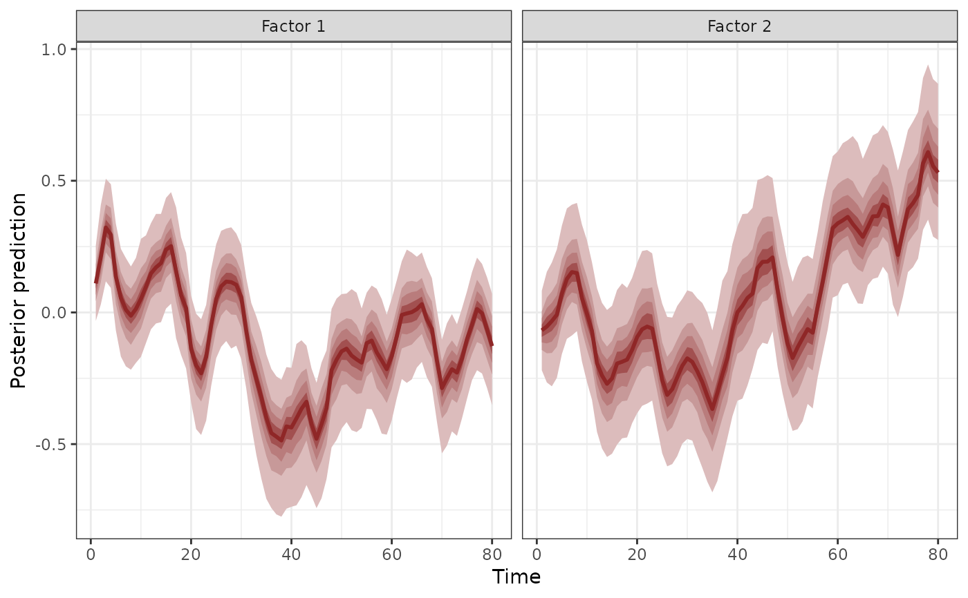#> # A tibble: 2 × 2
#>   Factor   Contribution
#>   <chr>           <dbl>
#> 1 Factor 1        0.534
#> 2 Factor 2        0.466

# Calculate correlations among the series
lvcors <- lv_correlations(mod)
names(lvcors)
#> [1] "mean_correlations"      "posterior_correlations"
lapply(lvcors, class)
#> $mean_correlations
#> [1] "matrix" "array" 
#> 
#> $posterior_correlations
#> [1] "list"
#> 

# Recommended: use residual_cor() instead
lvcors <- residual_cor(mod)
names(lvcors)
#>  [1] "cor"        "cor_lower"  "cor_upper"  "sig_cor"    "cov"       
#>  [6] "prec"       "prec_lower" "prec_upper" "sig_prec"   "trace"     
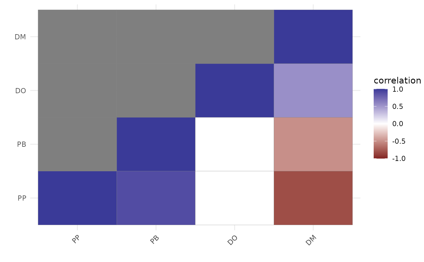
lvcors$cor
#>            DM         DO         PB          PP
#> DM  1.0000000 0.54925545 -0.4794042 -0.79837885
#> DO  0.5492555 1.00000000  0.4290647  0.01890233
#> PB -0.4794042 0.42906470  1.0000000  0.89413740
#> PP -0.7983788 0.01890233  0.8941374  1.00000000

# Plot credible correlations as a matrix
plot(lvcors, cluster = TRUE)


# \dontshow{
# For R CMD check: make sure any open connections are closed afterward
closeAllConnections()
# }
# }