Overview of the mvgam package

The purpose of this vignette is to give a general overview of the mvgam package and its primary functions.

Dynamic GAMs

mvgam is designed to propagate unobserved temporal processes to capture latent dynamics in the observed time series. This works in a state-space format, with the temporal trend evolving independently of the observation process. An introduction to the package and some worked examples are also shown in this seminar: Ecological Forecasting with Dynamic Generalized Additive Models. Briefly, assume \(\tilde{\boldsymbol{y}}_{i,t}\) is the conditional expectation of response variable \(\boldsymbol{i}\) at time \(\boldsymbol{t}\). Assuming \(\boldsymbol{y_i}\) is drawn from an exponential distribution with an invertible link function, the linear predictor for a multivariate Dynamic GAM can be written as:

\[for~i~in~1:N_{series}~...\] \[for~t~in~1:N_{timepoints}~...\]

\[g^{-1}(\tilde{\boldsymbol{y}}_{i,t})=\alpha_{i}+\sum\limits_{j=1}^J\boldsymbol{s}_{i,j,t}\boldsymbol{x}_{j,t}+\boldsymbol{z}_{i,t}\,,\] Here \(\alpha\) are the unknown intercepts, the \(\boldsymbol{s}\)’s are unknown smooth functions of covariates (\(\boldsymbol{x}\)’s), which can potentially vary among the response series, and \(\boldsymbol{z}\) are dynamic latent processes. Each smooth function \(\boldsymbol{s_j}\) is composed of basis expansions whose coefficients, which must be estimated, control the functional relationship between \(\boldsymbol{x}_{j}\) and \(g^{-1}(\tilde{\boldsymbol{y}})\). The size of the basis expansion limits the smooth’s potential complexity. A larger set of basis functions allows greater flexibility. For more information on GAMs and how they can smooth through data, see this blogpost on how to interpret nonlinear effects from Generalized Additive Models.

Several advantages of GAMs are that they can model a diversity of response families, including discrete distributions (i.e. Poisson, Negative Binomial, Gamma) that accommodate common ecological features such as zero-inflation or overdispersion, and that they can be formulated to include hierarchical smoothing for multivariate responses. mvgam supports a number of different observation families, which are summarized below:

Supported observation families

Distribution	Function	Support	Extra parameter(s)
Gaussian (identity link)	`gaussian()`	Real values in \((-\infty, \infty)\)	\(\sigma\)
Student’s T (identity link)	`student-t()`	Heavy-tailed real values in \((-\infty, \infty)\)	\(\sigma\), \(\nu\)
LogNormal (identity link)	`lognormal()`	Positive real values in \([0, \infty)\)	\(\sigma\)
Gamma (log link)	`Gamma()`	Positive real values in \([0, \infty)\)	\(\alpha\)
Beta (logit link)	`betar()`	Real values (proportional) in \([0,1]\)	\(\phi\)
Bernoulli (logit link)	`bernoulli()`	Binary data in \({0,1}\)	-
Poisson (log link)	`poisson()`	Non-negative integers in \((0,1,2,...)\)	-
Negative Binomial2 (log link)	`nb()`	Non-negative integers in \((0,1,2,...)\)	\(\phi\)
Binomial (logit link)	`binomial()`	Non-negative integers in \((0,1,2,...)\)	-
Beta-Binomial (logit link)	`beta_binomial()`	Non-negative integers in \((0,1,2,...)\)	\(\phi\)
Poisson Binomial N-mixture (log link)	`nmix()`	Non-negative integers in \((0,1,2,...)\)	-

For all supported observation families, any extra parameters that need to be estimated (i.e. the \(\sigma\) in a Gaussian model or the \(\phi\) in a Negative Binomial model) are by default estimated independently for each series. However, users can opt to force all series to share extra observation parameters using share_obs_params = TRUE in mvgam(). Note that default link functions cannot currently be changed.

Supported temporal dynamic processes

The dynamic processes can take a wide variety of forms, some of which can be multivariate to allow the different time series to interact or be correlated. When using the mvgam() function, the user chooses between different process models with the trend_model argument. Available process models are described in detail below.

Independent Random Walks

Use trend_model = 'RW' or trend_model = RW() to set up a model where each series in data has independent latent temporal dynamics of the form:

\[\begin{align*} z_{i,t} & \sim \text{Normal}(z_{i,t-1}, \sigma_i) \end{align*}\]

Process error parameters \(\sigma\) are modeled independently for each series. If a moving average process is required, use trend_model = RW(ma = TRUE) to set up the following:

\[\begin{align*} z_{i,t} & = z_{i,t-1} + \theta_i * error_{i,t-1} + error_{i,t} \\ error_{i,t} & \sim \text{Normal}(0, \sigma_i) \end{align*}\]

Moving average coefficients \(\theta\) are independently estimated for each series and will be forced to be stationary by default \((abs(\theta)<1)\). Only moving averages of order \(q=1\) are currently allowed.

Multivariate Random Walks

If more than one series is included in data \((N_{series} > 1)\), a multivariate Random Walk can be set up using trend_model = RW(cor = TRUE), resulting in the following:

\[\begin{align*} z_{t} & \sim \text{MVNormal}(z_{t-1}, \Sigma) \end{align*}\]

Where the latent process estimate \(z_t\) now takes the form of a vector. The covariance matrix \(\Sigma\) will capture contemporaneously correlated process errors. It is parameterised using a Cholesky factorization, which requires priors on the series-level variances \(\sigma\) and on the strength of correlations using Stan’s lkj_corr_cholesky distribution.

Moving average terms can also be included for multivariate random walks, in which case the moving average coefficients \(\theta\) will be parameterised as an \(N_{series} * N_{series}\) matrix

Autoregressive processes

Autoregressive models up to \(p=3\), in which the autoregressive coefficients are estimated independently for each series, can be used by specifying trend_model = 'AR1', trend_model = 'AR2', trend_model = 'AR3', or trend_model = AR(p = 1, 2, or 3). For example, a univariate AR(1) model takes the form:

\[\begin{align*} z_{i,t} & \sim \text{Normal}(ar1_i * z_{i,t-1}, \sigma_i) \end{align*}\]

All options are the same as for Random Walks, but additional options will be available for placing priors on the autoregressive coefficients. By default, these coefficients will not be forced into stationarity, but users can impose this restriction by changing the upper and lower bounds on their priors. See ?get_mvgam_priors for more details.

Vector Autoregressive processes

A Vector Autoregression of order \(p=1\) can be specified if \(N_{series} > 1\) using trend_model = 'VAR1' or trend_model = VAR(). A VAR(1) model takes the form:

\[\begin{align*} z_{t} & \sim \text{Normal}(A * z_{t-1}, \Sigma) \end{align*}\]

Where \(A\) is an \(N_{series} * N_{series}\) matrix of autoregressive coefficients in which the diagonals capture lagged self-dependence (i.e. the effect of a process at time \(t\) on its own estimate at time \(t+1\)), while off-diagonals capture lagged cross-dependence (i.e. the effect of a process at time \(t\) on the process for another series at time \(t+1\)). By default, the covariance matrix \(\Sigma\) will assume no process error covariance by fixing the off-diagonals to \(0\). To allow for correlated errors, use trend_model = 'VAR1cor' or trend_model = VAR(cor = TRUE). A moving average of order \(q=1\) can also be included using trend_model = VAR(ma = TRUE, cor = TRUE).

Note that for all VAR models, stationarity of the process is enforced with a structured prior distribution that is described in detail in Heaps 2022

Heaps, Sarah E. “Enforcing stationarity through the prior in vector autoregressions.” Journal of Computational and Graphical Statistics 32.1 (2023): 74-83.

Gaussian Processes

The final option for modelling temporal dynamics is to use a Gaussian Process with squared exponential kernel. These are set up independently for each series (there is currently no multivariate GP option), using trend_model = 'GP'. The dynamics for each latent process are modelled as:

\[\begin{align*} z & \sim \text{MVNormal}(0, \Sigma_{error}) \\ \Sigma_{error}[t_i, t_j] & = \alpha^2 * exp(-0.5 * ((|t_i - t_j| / \rho))^2) \end{align*}\]

The latent dynamic process evolves from a complex, high-dimensional Multivariate Normal distribution which depends on \(\rho\) (often called the length scale parameter) to control how quickly the correlations between the model’s errors decay as a function of time. For these models, covariance decays exponentially fast with the squared distance (in time) between the observations. The functions also depend on a parameter \(\alpha\), which controls the marginal variability of the temporal function at all points; in other words it controls how much the GP term contributes to the linear predictor. mvgam capitalizes on some advances that allow GPs to be approximated using Hilbert space basis functions, which considerably speed up computation at little cost to accuracy or prediction performance.

Piecewise logistic and linear trends

Modeling growth for many types of time series is often similar to modeling population growth in natural ecosystems, where there series exhibits nonlinear growth that saturates at some particular carrying capacity. The logistic trend model available in {mvgam} allows for a time-varying capacity \(C(t)\) as well as a non-constant growth rate. Changes in the base growth rate \(k\) are incorporated by explicitly defining changepoints throughout the training period where the growth rate is allowed to vary. The changepoint vector \(a\) is represented as a vector of 1s and 0s, and the rate of growth at time \(t\) is represented as \(k+a(t)^T\delta\). Potential changepoints are selected uniformly across the training period, and the number of changepoints, as well as the flexibility of the potential rate changes at these changepoints, can be controlled using trend_model = PW(). The full piecewise logistic growth model is then:

\[\begin{align*} z_t & = \frac{C_t}{1 + \exp(-(k+a(t)^T\delta)(t-(m+a(t)^T\gamma)))} \end{align*}\]

For time series that do not appear to exhibit saturating growth, a piece-wise constant rate of growth can often provide a useful trend model. The piecewise linear trend is defined as:

\[\begin{align*} z_t & = (k+a(t)^T\delta)t + (m+a(t)^T\gamma) \end{align*}\]

In both trend models, \(m\) is an offset parameter that controls the trend intercept. Because of this parameter, it is not recommended that you include an intercept in your observation formula because this will not be identifiable. You can read about the full description of piecewise linear and logistic trends in this paper by Taylor and Letham.

Sean J. Taylor and Benjamin Letham. “Forecasting at scale.” The American Statistician 72.1 (2018): 37-45.

Continuous time AR(1) processes

Most trend models in the mvgam() function expect time to be measured in regularly-spaced, discrete intervals (i.e. one measurement per week, or one per year for example). But some time series are taken at irregular intervals and we’d like to model autoregressive properties of these. The trend_model = CAR() can be useful to set up these models, which currently only support autoregressive processes of order 1. The evolution of the latent dynamic process follows the form:

\[\begin{align*} z_{i,t} & \sim \text{Normal}(ar1_i^{distance} * z_{i,t-1}, \sigma_i) \end{align*}\]

Where \(distance\) is a vector of non-negative measurements of the time differences between successive observations. See the Examples section in ?CAR for an illustration of how to set these models up.

Regression formulae

mvgam supports an observation model regression formula, built off the mgcv package, as well as an optional process model regression formula. The formulae supplied to are exactly like those supplied to glm() except that smooth terms, s(), te(), ti() and t2(), time-varying effects using dynamic(), monotonically increasing (using s(x, bs = 'moi')) or decreasing splines (using s(x, bs = 'mod'); see ?smooth.construct.moi.smooth.spec for details), as well as Gaussian Process functions using gp(), can be added to the right hand side (and . is not supported in mvgam formulae). See ?mvgam_formulae for more guidance.

For setting up State-Space models, the optional process model formula can be used (see the State-Space model vignette and the shared latent states vignette for guidance on using trend formulae).

Example time series data

The ‘portal_data’ object contains time series of rodent captures from the Portal Project, a long-term monitoring study based near the town of Portal, Arizona. Researchers have been operating a standardized set of baited traps within 24 experimental plots at this site since the 1970’s. Sampling follows the lunar monthly cycle, with observations occurring on average about 28 days apart. However, missing observations do occur due to difficulties accessing the site (weather events, COVID disruptions etc…). You can read about the full sampling protocol in this preprint by Ernest et al on the Biorxiv.

data("portal_data")

As the data come pre-loaded with the mvgam package, you can read a little about it in the help page using ?portal_data. Before working with data, it is important to inspect how the data are structured, first using head:

head(portal_data)
#>   moon DM DO PP OT year month mintemp precipitation     ndvi
#> 1  329 10  6  0  2 2004     1  -9.710          37.8 1.465889
#> 2  330 14  8  1  0 2004     2  -5.924           8.7 1.558507
#> 3  331  9  1  2  1 2004     3  -0.220          43.5 1.337817
#> 4  332 NA NA NA NA 2004     4   1.931          23.9 1.658913
#> 5  333 15  8 10  1 2004     5   6.568           0.9 1.853656
#> 6  334 NA NA NA NA 2004     6  11.590           1.4 1.761330

But the glimpse function in dplyr is also useful for understanding how variables are structured

dplyr::glimpse(portal_data)
#> Rows: 199
#> Columns: 10
#> $ moon          <int> 329, 330, 331, 332, 333, 334, 335, 336, 337, 338, 339, 3…
#> $ DM            <int> 10, 14, 9, NA, 15, NA, NA, 9, 5, 8, NA, 14, 7, NA, NA, 9…
#> $ DO            <int> 6, 8, 1, NA, 8, NA, NA, 3, 3, 4, NA, 3, 8, NA, NA, 3, NA…
#> $ PP            <int> 0, 1, 2, NA, 10, NA, NA, 16, 18, 12, NA, 3, 2, NA, NA, 1…
#> $ OT            <int> 2, 0, 1, NA, 1, NA, NA, 1, 0, 0, NA, 2, 1, NA, NA, 1, NA…
#> $ year          <int> 2004, 2004, 2004, 2004, 2004, 2004, 2004, 2004, 2004, 20…
#> $ month         <int> 1, 2, 3, 4, 5, 6, 7, 8, 9, 10, 11, 12, 1, 2, 3, 4, 5, 6,…
#> $ mintemp       <dbl> -9.710, -5.924, -0.220, 1.931, 6.568, 11.590, 14.370, 16…
#> $ precipitation <dbl> 37.8, 8.7, 43.5, 23.9, 0.9, 1.4, 20.3, 91.0, 60.5, 25.2,…
#> $ ndvi          <dbl> 1.4658889, 1.5585069, 1.3378172, 1.6589129, 1.8536561, 1…

We will focus analyses on the time series of captures for one specific rodent species, the Desert Pocket Mouse Chaetodipus penicillatus. This species is interesting in that it goes into a kind of “hibernation” during the colder months, leading to very low captures during the winter period

Manipulating data for modelling

Manipulating the data into a ‘long’ format is necessary for modelling in mvgam. By ‘long’ format, we mean that each series x time observation needs to have its own entry in the dataframe or list object that we wish to use as data for modelling. A simple example can be viewed by simulating data using the sim_mvgam function. See ?sim_mvgam for more details

data <- sim_mvgam(n_series = 4, T = 24)
head(data$data_train, 12)
#>    y season year   series time
#> 1  2      1    1 series_1    1
#> 2  0      1    1 series_2    1
#> 3  1      1    1 series_3    1
#> 4  1      1    1 series_4    1
#> 5  0      2    1 series_1    2
#> 6  0      2    1 series_2    2
#> 7  1      2    1 series_3    2
#> 8  0      2    1 series_4    2
#> 9  0      3    1 series_1    3
#> 10 0      3    1 series_2    3
#> 11 0      3    1 series_3    3
#> 12 0      3    1 series_4    3

Notice how we have four different time series in these simulated data, but we do not spread the outcome values into different columns. Rather, there is only a single column for the outcome variable, labelled y in these simulated data. We also must supply a variable labelled time to ensure the modelling software knows how to arrange the time series when building models. This setup still allows us to formulate multivariate time series models, as you can see in the State-Space vignette. Below are the steps needed to shape our portal_data object into the correct form. First, we create a time variable, select the column representing counts of our target species (PP), and select appropriate variables that we can use as predictors

portal_data %>%
  
  # mvgam requires a 'time' variable be present in the data to index
  # the temporal observations. This is especially important when tracking 
  # multiple time series. In the Portal data, the 'moon' variable indexes the
  # lunar monthly timestep of the trapping sessions
  dplyr::mutate(time = moon - (min(moon)) + 1) %>%
  
  # We can also provide a more informative name for the outcome variable, which 
  # is counts of the 'PP' species (Chaetodipus penicillatus) across all control
  # plots
  dplyr::mutate(count = PP) %>%
  
  # The other requirement for mvgam is a 'series' variable, which needs to be a
  # factor variable to index which time series each row in the data belongs to.
  # Again, this is more useful when you have multiple time series in the data
  dplyr::mutate(series = as.factor('PP')) %>%
  
  # Select the variables of interest to keep in the model_data
  dplyr::select(series, year, time, count, mintemp, ndvi) -> model_data

The data now contain six variables:
series, a factor indexing which time series each observation belongs to
year, the year of sampling
time, the indicator of which time step each observation belongs to
count, the response variable representing the number of captures of the species PP in each sampling observation
mintemp, the monthly average minimum temperature at each time step
ndvi, the monthly average Normalized Difference Vegetation Index at each time step

Now check the data structure again

head(model_data)
#>   series year time count mintemp     ndvi
#> 1     PP 2004    1     0  -9.710 1.465889
#> 2     PP 2004    2     1  -5.924 1.558507
#> 3     PP 2004    3     2  -0.220 1.337817
#> 4     PP 2004    4    NA   1.931 1.658913
#> 5     PP 2004    5    10   6.568 1.853656
#> 6     PP 2004    6    NA  11.590 1.761330

dplyr::glimpse(model_data)
#> Rows: 199
#> Columns: 6
#> $ series  <fct> PP, PP, PP, PP, PP, PP, PP, PP, PP, PP, PP, PP, PP, PP, PP, PP…
#> $ year    <int> 2004, 2004, 2004, 2004, 2004, 2004, 2004, 2004, 2004, 2004, 20…
#> $ time    <dbl> 1, 2, 3, 4, 5, 6, 7, 8, 9, 10, 11, 12, 13, 14, 15, 16, 17, 18,…
#> $ count   <int> 0, 1, 2, NA, 10, NA, NA, 16, 18, 12, NA, 3, 2, NA, NA, 13, NA,…
#> $ mintemp <dbl> -9.710, -5.924, -0.220, 1.931, 6.568, 11.590, 14.370, 16.520, …
#> $ ndvi    <dbl> 1.4658889, 1.5585069, 1.3378172, 1.6589129, 1.8536561, 1.76132…

You can also summarize multiple variables, which is helpful to search for data ranges and identify missing values

summary(model_data)
#>  series        year           time           count          mintemp       
#>  PP:199   Min.   :2004   Min.   :  1.0   Min.   : 0.00   Min.   :-24.000  
#>           1st Qu.:2008   1st Qu.: 50.5   1st Qu.: 2.50   1st Qu.: -3.884  
#>           Median :2012   Median :100.0   Median :12.00   Median :  2.130  
#>           Mean   :2012   Mean   :100.0   Mean   :15.14   Mean   :  3.504  
#>           3rd Qu.:2016   3rd Qu.:149.5   3rd Qu.:24.00   3rd Qu.: 12.310  
#>           Max.   :2020   Max.   :199.0   Max.   :65.00   Max.   : 18.140  
#>                                          NA's   :36                       
#>       ndvi       
#>  Min.   :0.2817  
#>  1st Qu.:1.0741  
#>  Median :1.3501  
#>  Mean   :1.4709  
#>  3rd Qu.:1.8178  
#>  Max.   :3.9126  
#>

We have some NAs in our response variable count. Let’s visualize the data as a heatmap to get a sense of where these are distributed (NAs are shown as red bars in the below plot)

image(is.na(t(model_data %>%
                dplyr::arrange(dplyr::desc(time)))), axes = F,
      col = c('grey80', 'darkred'))
axis(3, at = seq(0,1, len = NCOL(model_data)), labels = colnames(model_data))

These observations will generally be thrown out by most modelling packages in . But as you will see when we work through the tutorials, mvgam keeps these in the data so that predictions can be automatically returned for the full dataset. The time series and some of its descriptive features can be plotted using plot_mvgam_series():

plot_mvgam_series(data = model_data, series = 1, y = 'count')

GLMs with temporal random effects

Our first task will be to fit a Generalized Linear Model (GLM) that can adequately capture the features of our count observations (integer data, lower bound at zero, missing values) while also attempting to model temporal variation. We are almost ready to fit our first model, which will be a GLM with Poisson observations, a log link function and random (hierarchical) intercepts for year. This will allow us to capture our prior belief that, although each year is unique, having been sampled from the same population of effects, all years are connected and thus might contain valuable information about one another. This will be done by capitalizing on the partial pooling properties of hierarchical models. Hierarchical (also known as random) effects offer many advantages when modelling data with grouping structures (i.e. multiple species, locations, years etc…). The ability to incorporate these in time series models is a huge advantage over traditional models such as ARIMA or Exponential Smoothing. But before we fit the model, we will need to convert year to a factor so that we can use a random effect basis in mvgam. See ?smooth.terms and ?smooth.construct.re.smooth.spec for details about the re basis construction that is used by both mvgam and mgcv

model_data %>%
  
  # Create a 'year_fac' factor version of 'year'
  dplyr::mutate(year_fac = factor(year)) -> model_data

Preview the dataset to ensure year is now a factor with a unique factor level for each year in the data

dplyr::glimpse(model_data)
#> Rows: 199
#> Columns: 7
#> $ series   <fct> PP, PP, PP, PP, PP, PP, PP, PP, PP, PP, PP, PP, PP, PP, PP, P…
#> $ year     <int> 2004, 2004, 2004, 2004, 2004, 2004, 2004, 2004, 2004, 2004, 2…
#> $ time     <dbl> 1, 2, 3, 4, 5, 6, 7, 8, 9, 10, 11, 12, 13, 14, 15, 16, 17, 18…
#> $ count    <int> 0, 1, 2, NA, 10, NA, NA, 16, 18, 12, NA, 3, 2, NA, NA, 13, NA…
#> $ mintemp  <dbl> -9.710, -5.924, -0.220, 1.931, 6.568, 11.590, 14.370, 16.520,…
#> $ ndvi     <dbl> 1.4658889, 1.5585069, 1.3378172, 1.6589129, 1.8536561, 1.7613…
#> $ year_fac <fct> 2004, 2004, 2004, 2004, 2004, 2004, 2004, 2004, 2004, 2004, 2…
levels(model_data$year_fac)
#>  [1] "2004" "2005" "2006" "2007" "2008" "2009" "2010" "2011" "2012" "2013"
#> [11] "2014" "2015" "2016" "2017" "2018" "2019" "2020"

We are now ready for our first mvgam model. The syntax will be familiar to users who have previously built models with mgcv. But for a refresher, see ?formula.gam and the examples in ?gam. Random effects can be specified using the s wrapper with the re basis. Note that we can also suppress the primary intercept using the usual R formula syntax - 1. mvgam has a number of possible observation families that can be used, see ?mvgam_families for more information. We will use Stan as the fitting engine, which deploys Hamiltonian Monte Carlo (HMC) for full Bayesian inference. By default, 4 HMC chains will be run using a warmup of 500 iterations and collecting 500 posterior samples from each chain. The package will also aim to use the Cmdstan backend when possible, so it is recommended that users have an up-to-date installation of Cmdstan and the associated cmdstanr interface on their machines (note that you can set the backend yourself using the backend argument: see ?mvgam for details). Interested users should consult the Stan user’s guide for more information about the software and the enormous variety of models that can be tackled with HMC.

model1 <- mvgam(count ~ s(year_fac, bs = 're') - 1,
                family = poisson(),
                data = model_data)

The model can be described mathematically for each timepoint \(t\) as follows: \[\begin{align*} \boldsymbol{count}_t & \sim \text{Poisson}(\lambda_t) \\ log(\lambda_t) & = \beta_{year[year_t]} \\ \beta_{year} & \sim \text{Normal}(\mu_{year}, \sigma_{year}) \end{align*}\]

Where the \(\beta_{year}\) effects are drawn from a population distribution that is parameterized by a common mean \((\mu_{year})\) and variance \((\sigma_{year})\). Priors on most of the model parameters can be interrogated and changed using similar functionality to the options available in brms. For example, the default priors on \((\mu_{year})\) and \((\sigma_{year})\) can be viewed using the following code:

get_mvgam_priors(count ~ s(year_fac, bs = 're') - 1,
                 family = poisson(),
                 data = model_data)
#>                      param_name param_length           param_info
#> 1             vector[1] mu_raw;            1 s(year_fac) pop mean
#> 2 vector<lower=0>[1] sigma_raw;            1   s(year_fac) pop sd
#>                               prior                example_change
#> 1            mu_raw ~ std_normal();  mu_raw ~ normal(0.05, 0.35);
#> 2 sigma_raw ~ student_t(3, 0, 2.5); sigma_raw ~ exponential(0.4);
#>   new_lowerbound new_upperbound
#> 1             NA             NA
#> 2             NA             NA

See examples in ?get_mvgam_priors to find out different ways that priors can be altered. Once the model has finished, the first step is to inspect the summary to ensure no major diagnostic warnings have been produced and to quickly summarise posterior distributions for key parameters

summary(model1)
#> GAM formula:
#> count ~ s(year_fac, bs = "re") - 1
#> 
#> Family:
#> poisson
#> 
#> Link function:
#> log
#> 
#> Trend model:
#> None
#> 
#> N series:
#> 1 
#> 
#> N timepoints:
#> 199 
#> 
#> Status:
#> Fitted using Stan 
#> 4 chains, each with iter = 1000; warmup = 500; thin = 1 
#> Total post-warmup draws = 2000
#> 
#> 
#> GAM coefficient (beta) estimates:
#>                2.5% 50% 97.5% Rhat n_eff
#> s(year_fac).1   1.8 2.1   2.3 1.00  2329
#> s(year_fac).2   2.5 2.7   2.8 1.00  3391
#> s(year_fac).3   3.0 3.1   3.2 1.00  3678
#> s(year_fac).4   3.1 3.3   3.4 1.00  2502
#> s(year_fac).5   1.9 2.1   2.3 1.00  3208
#> s(year_fac).6   1.5 1.7   2.0 1.00  2729
#> s(year_fac).7   1.8 2.0   2.3 1.00  2280
#> s(year_fac).8   2.8 3.0   3.1 1.00  2928
#> s(year_fac).9   3.1 3.2   3.4 1.00  2409
#> s(year_fac).10  2.6 2.8   2.9 1.00  3752
#> s(year_fac).11  3.0 3.1   3.2 1.00  2762
#> s(year_fac).12  3.1 3.2   3.3 1.00  2621
#> s(year_fac).13  2.0 2.3   2.5 1.00  2785
#> s(year_fac).14  2.5 2.6   2.8 1.00  3025
#> s(year_fac).15  2.0 2.2   2.4 1.00  2693
#> s(year_fac).16  1.9 2.1   2.3 1.00  3452
#> s(year_fac).17 -0.3 1.0   1.9 1.01   419
#> 
#> GAM group-level estimates:
#>                   2.5% 50% 97.5% Rhat n_eff
#> mean(s(year_fac)) 2.00 2.4   2.7 1.04   218
#> sd(s(year_fac))   0.47 0.7   1.1 1.02   233
#> 
#> Approximate significance of GAM smooths:
#>              edf Ref.df Chi.sq p-value    
#> s(year_fac) 13.6     17  24257  <2e-16 ***
#> ---
#> Signif. codes:  0 '***' 0.001 '**' 0.01 '*' 0.05 '.' 0.1 ' ' 1
#> 
#> Stan MCMC diagnostics:
#> n_eff / iter looks reasonable for all parameters
#> Rhat looks reasonable for all parameters
#> 0 of 2000 iterations ended with a divergence (0%)
#> 0 of 2000 iterations saturated the maximum tree depth of 12 (0%)
#> E-FMI indicated no pathological behavior
#> 
#> Samples were drawn using NUTS(diag_e) at Wed May 08 9:23:14 AM 2024.
#> For each parameter, n_eff is a crude measure of effective sample size,
#> and Rhat is the potential scale reduction factor on split MCMC chains
#> (at convergence, Rhat = 1)

The diagnostic messages at the bottom of the summary show that the HMC sampler did not encounter any problems or difficult posterior spaces. This is a good sign. Posterior distributions for model parameters can be extracted in any way that an object of class brmsfit can (see ?mvgam::mvgam_draws for details). For example, we can extract the coefficients related to the GAM linear predictor (i.e. the \(\beta\)’s) into a data.frame using:

beta_post <- as.data.frame(model1, variable = 'betas')
dplyr::glimpse(beta_post)
#> Rows: 2,000
#> Columns: 17
#> $ `s(year_fac).1`  <dbl> 2.26471, 2.28646, 1.88877, 2.13797, 2.13292, 1.90150,…
#> $ `s(year_fac).2`  <dbl> 2.60161, 2.55260, 2.83022, 2.57911, 2.73152, 2.63560,…
#> $ `s(year_fac).3`  <dbl> 3.02223, 3.11011, 3.07508, 3.05916, 3.15232, 3.05806,…
#> $ `s(year_fac).4`  <dbl> 3.23014, 3.26369, 3.30038, 3.32252, 3.16570, 3.29277,…
#> $ `s(year_fac).5`  <dbl> 2.20354, 2.11918, 2.13862, 2.23733, 2.11541, 2.24504,…
#> $ `s(year_fac).6`  <dbl> 1.58277, 1.86747, 1.80698, 1.75366, 1.61760, 1.82839,…
#> $ `s(year_fac).7`  <dbl> 2.06464, 2.18970, 1.93242, 2.20787, 2.10049, 2.15573,…
#> $ `s(year_fac).8`  <dbl> 3.00108, 2.84201, 2.82476, 3.13209, 2.82666, 3.03052,…
#> $ `s(year_fac).9`  <dbl> 3.12485, 3.35995, 3.16244, 3.28071, 3.30909, 3.30901,…
#> $ `s(year_fac).10` <dbl> 2.75109, 2.75129, 2.70531, 2.87279, 2.65541, 2.84888,…
#> $ `s(year_fac).11` <dbl> 2.96471, 3.15959, 3.17329, 2.93121, 3.16503, 3.10468,…
#> $ `s(year_fac).12` <dbl> 3.21647, 3.16220, 3.21724, 3.19282, 3.07472, 3.17971,…
#> $ `s(year_fac).13` <dbl> 2.17085, 2.16766, 2.28339, 2.29180, 2.22491, 2.11617,…
#> $ `s(year_fac).14` <dbl> 2.82083, 2.54186, 2.49718, 2.79898, 2.52417, 2.76137,…
#> $ `s(year_fac).15` <dbl> 2.00444, 2.05338, 2.31112, 2.08922, 2.14740, 2.06587,…
#> $ `s(year_fac).16` <dbl> 1.88497, 2.07941, 2.15184, 2.18370, 2.02184, 2.14112,…
#> $ `s(year_fac).17` <dbl> 1.598580, 1.464190, 1.310510, 1.627650, 1.192140, 1.2…

With any model fitted in mvgam, the underlying Stan code can be viewed using the code function:

code(model1)
#> // Stan model code generated by package mvgam
#> data {
#>   int<lower=0> total_obs; // total number of observations
#>   int<lower=0> n; // number of timepoints per series
#>   int<lower=0> n_series; // number of series
#>   int<lower=0> num_basis; // total number of basis coefficients
#>   matrix[total_obs, num_basis] X; // mgcv GAM design matrix
#>   array[n, n_series] int<lower=0> ytimes; // time-ordered matrix (which col in X belongs to each [time, series] observation?)
#>   int<lower=0> n_nonmissing; // number of nonmissing observations
#>   array[n_nonmissing] int<lower=0> flat_ys; // flattened nonmissing observations
#>   matrix[n_nonmissing, num_basis] flat_xs; // X values for nonmissing observations
#>   array[n_nonmissing] int<lower=0> obs_ind; // indices of nonmissing observations
#> }
#> parameters {
#>   // raw basis coefficients
#>   vector[num_basis] b_raw;
#>   
#>   // random effect variances
#>   vector<lower=0>[1] sigma_raw;
#>   
#>   // random effect means
#>   vector[1] mu_raw;
#> }
#> transformed parameters {
#>   // basis coefficients
#>   vector[num_basis] b;
#>   b[1 : 17] = mu_raw[1] + b_raw[1 : 17] * sigma_raw[1];
#> }
#> model {
#>   // prior for random effect population variances
#>   sigma_raw ~ student_t(3, 0, 2.5);
#>   
#>   // prior for random effect population means
#>   mu_raw ~ std_normal();
#>   
#>   // prior (non-centred) for s(year_fac)...
#>   b_raw[1 : 17] ~ std_normal();
#>   {
#>     // likelihood functions
#>     flat_ys ~ poisson_log_glm(flat_xs, 0.0, b);
#>   }
#> }
#> generated quantities {
#>   vector[total_obs] eta;
#>   matrix[n, n_series] mus;
#>   array[n, n_series] int ypred;
#>   
#>   // posterior predictions
#>   eta = X * b;
#>   for (s in 1 : n_series) {
#>     mus[1 : n, s] = eta[ytimes[1 : n, s]];
#>     ypred[1 : n, s] = poisson_log_rng(mus[1 : n, s]);
#>   }
#> }

Plotting effects and residuals

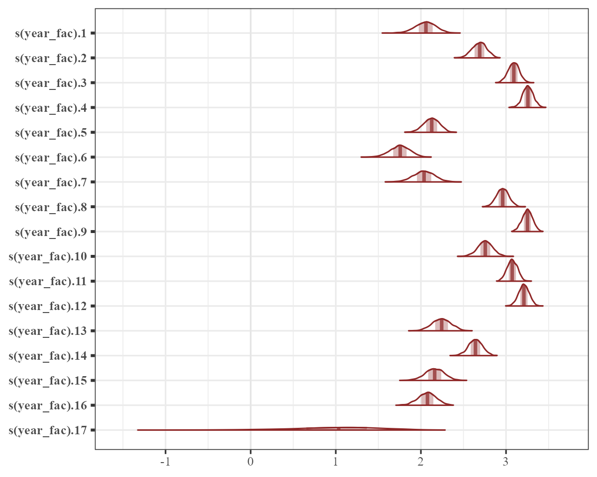
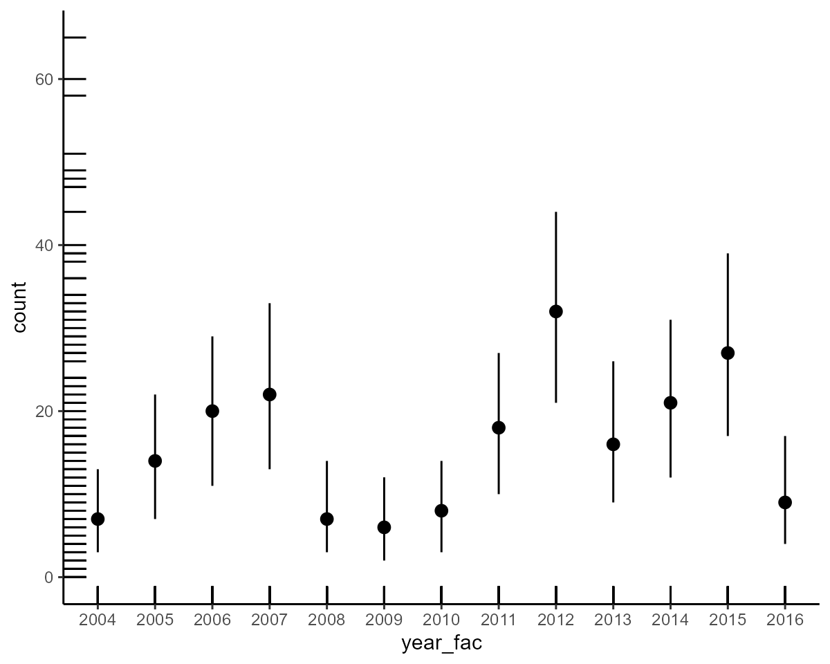
Now for interrogating the model. We can get some sense of the variation in yearly intercepts from the summary above, but it is easier to understand them using targeted plots. Plot posterior distributions of the temporal random effects using plot.mvgam with type = 're'. See ?plot.mvgam for more details about the types of plots that can be produced from fitted mvgam objects

plot(model1, type = 're')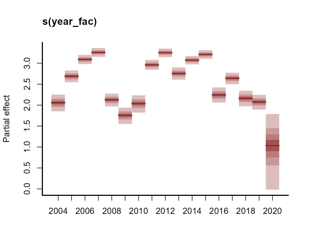

`bayesplot` support

We can also capitalize on most of the useful MCMC plotting functions from the bayesplot package to visualize posterior distributions and diagnostics (see ?mvgam::mcmc_plot.mvgam for details):

mcmc_plot(object = model1,
          variable = 'betas',
          type = 'areas')

We can also use the wide range of posterior checking functions available in bayesplot (see ?mvgam::ppc_check.mvgam for details):

pp_check(object = model1)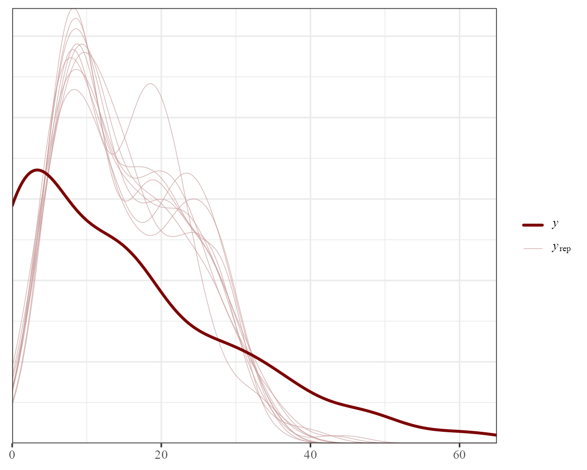
#> Using 10 posterior draws for ppc type 'dens_overlay' by default.
#> Warning in pp_check.mvgam(object = model1): NA responses are not shown in
#> 'pp_check'.

pp_check(model1, type = "rootogram")
#> Using all posterior draws for ppc type 'rootogram' by default.
#> Warning in pp_check.mvgam(model1, type = "rootogram"): NA responses are not
#> shown in 'pp_check'.

There is clearly some variation in these yearly intercept estimates. But how do these translate into time-varying predictions? To understand this, we can plot posterior hindcasts from this model for the training period using plot.mvgam with type = 'forecast'

plot(model1, type = 'forecast')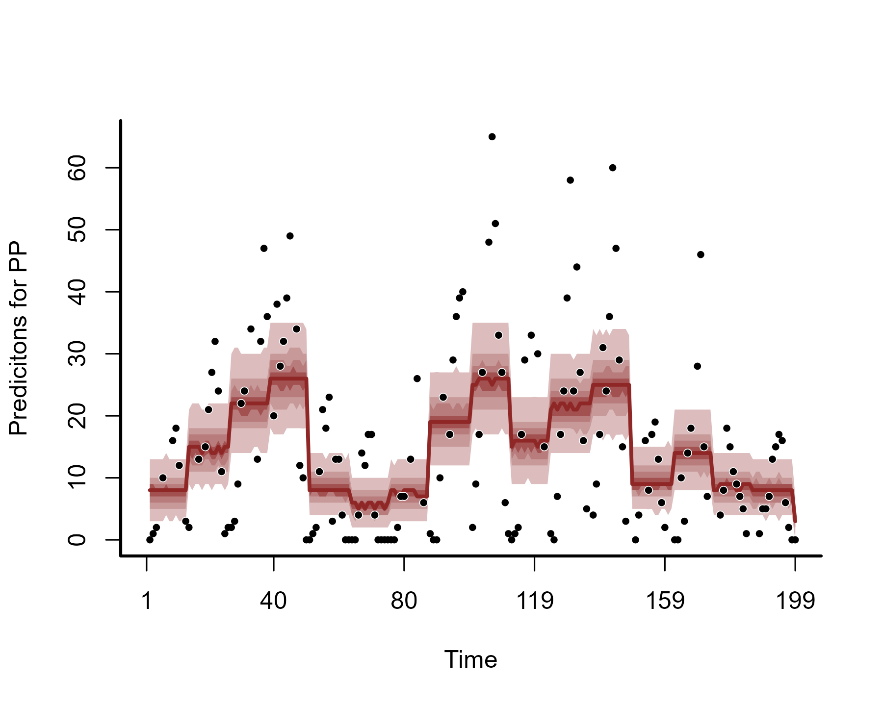

If you wish to extract these hindcasts for other downstream analyses, the hindcast function can be used. This will return a list object of class mvgam_forecast. In the hindcasts slot, a matrix of posterior retrodictions will be returned for each series in the data (only one series in our example):

hc <- hindcast(model1)
str(hc)
#> List of 15
#>  $ call              :Class 'formula'  language count ~ s(year_fac, bs = "re") - 1
#>   .. ..- attr(*, ".Environment")=<environment: R_GlobalEnv> 
#>  $ trend_call        : NULL
#>  $ family            : chr "poisson"
#>  $ trend_model       : chr "None"
#>  $ drift             : logi FALSE
#>  $ use_lv            : logi FALSE
#>  $ fit_engine        : chr "stan"
#>  $ type              : chr "response"
#>  $ series_names      : chr "PP"
#>  $ train_observations:List of 1
#>   ..$ PP: int [1:199] 0 1 2 NA 10 NA NA 16 18 12 ...
#>  $ train_times       : num [1:199] 1 2 3 4 5 6 7 8 9 10 ...
#>  $ test_observations : NULL
#>  $ test_times        : NULL
#>  $ hindcasts         :List of 1
#>   ..$ PP: num [1:2000, 1:199] 6 10 3 12 6 7 6 3 6 2 ...
#>   .. ..- attr(*, "dimnames")=List of 2
#>   .. .. ..$ : NULL
#>   .. .. ..$ : chr [1:199] "ypred[1,1]" "ypred[2,1]" "ypred[3,1]" "ypred[4,1]" ...
#>  $ forecasts         : NULL
#>  - attr(*, "class")= chr "mvgam_forecast"

You can also extract these hindcasts on the linear predictor scale, which in this case is the log scale (our Poisson GLM used a log link function). Sometimes this can be useful for asking more targeted questions about drivers of variation:

hc <- hindcast(model1, type = 'link')
range(hc$hindcasts$PP)
#> [1] -1.94773  3.44074

Objects of class mvgam_forecast have an associated plot function as well:

plot(hc)

This plot can look a bit confusing as it seems like there is linear interpolation from the end of one year to the start of the next. But this is just due to the way the lines are automatically connected in base plots

In any regression analysis, a key question is whether the residuals show any patterns that can be indicative of un-modelled sources of variation. For GLMs, we can use a modified residual called the Dunn-Smyth, or randomized quantile, residual. Inspect Dunn-Smyth residuals from the model using plot.mvgam with type = 'residuals'

plot(model1, type = 'residuals')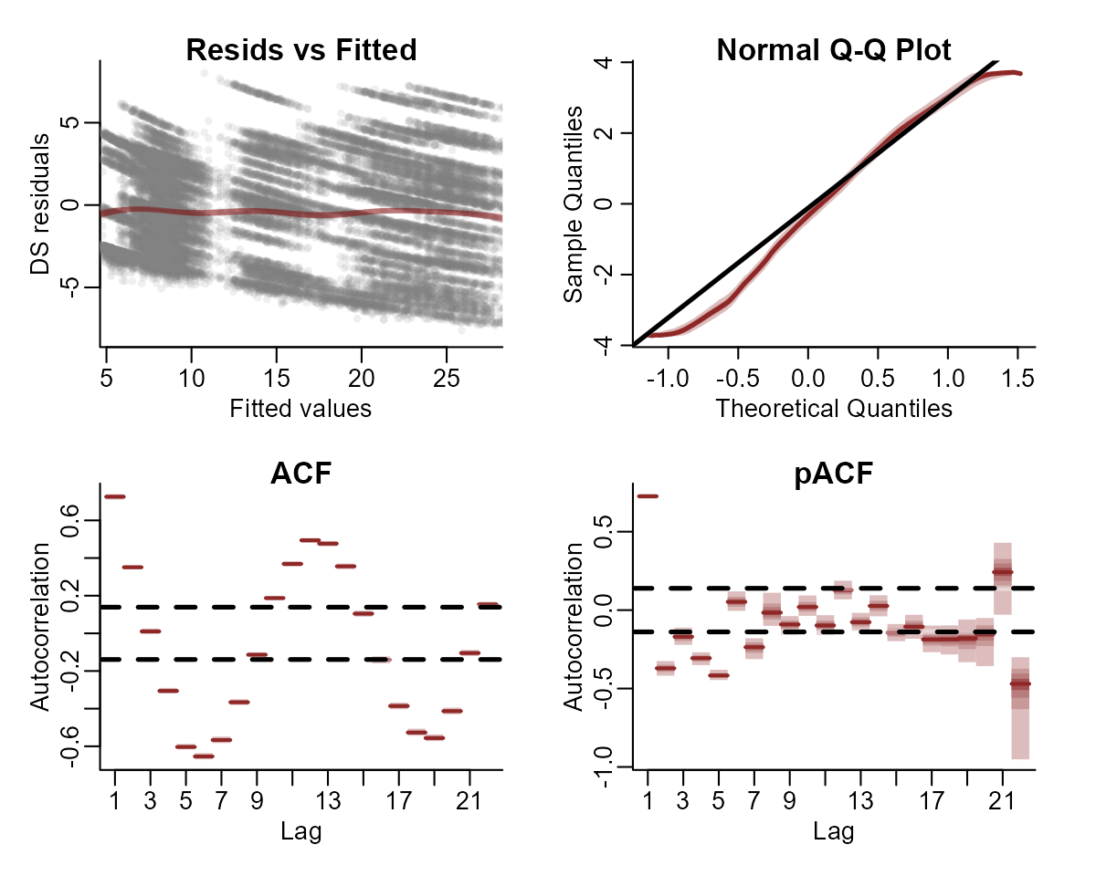

Automatic forecasting for new data

These temporal random effects do not have a sense of “time”. Because of this, each yearly random intercept is not restricted in some way to be similar to the previous yearly intercept. This drawback becomes evident when we predict for a new year. To do this, we can repeat the exercise above but this time will split the data into training and testing sets before re-running the model. We can then supply the test set as newdata. For splitting, we will make use of the filter function from dplyr

model_data %>% 
  dplyr::filter(time <= 160) -> data_train 
model_data %>% 
  dplyr::filter(time > 160) -> data_test

model1b <- mvgam(count ~ s(year_fac, bs = 're') - 1,
                family = poisson(),
                data = data_train,
                newdata = data_test)

Repeating the plots above gives insight into how the model’s hierarchical prior formulation provides all the structure needed to sample values for un-modelled years

plot(model1b, type = 're')

plot(model1b, type = 'forecast')
#> Out of sample DRPS:
#> 181.98880875

We can also view the test data in the forecast plot to see that the predictions do not capture the temporal variation in the test set

plot(model1b, type = 'forecast', newdata = data_test)
#> Out of sample DRPS:
#> 181.98880875

As with the hindcast function, we can use the forecast function to automatically extract the posterior distributions for these predictions. This also returns an object of class mvgam_forecast, but now it will contain both the hindcasts and forecasts for each series in the data:

fc <- forecast(model1b)
str(fc)
#> List of 16
#>  $ call              :Class 'formula'  language count ~ s(year_fac, bs = "re") - 1
#>   .. ..- attr(*, ".Environment")=<environment: R_GlobalEnv> 
#>  $ trend_call        : NULL
#>  $ family            : chr "poisson"
#>  $ family_pars       : NULL
#>  $ trend_model       : chr "None"
#>  $ drift             : logi FALSE
#>  $ use_lv            : logi FALSE
#>  $ fit_engine        : chr "stan"
#>  $ type              : chr "response"
#>  $ series_names      : Factor w/ 1 level "PP": 1
#>  $ train_observations:List of 1
#>   ..$ PP: int [1:160] 0 1 2 NA 10 NA NA 16 18 12 ...
#>  $ train_times       : num [1:160] 1 2 3 4 5 6 7 8 9 10 ...
#>  $ test_observations :List of 1
#>   ..$ PP: int [1:39] NA 0 0 10 3 14 18 NA 28 46 ...
#>  $ test_times        : num [1:39] 161 162 163 164 165 166 167 168 169 170 ...
#>  $ hindcasts         :List of 1
#>   ..$ PP: num [1:2000, 1:160] 7 9 6 10 5 8 14 15 8 11 ...
#>   .. ..- attr(*, "dimnames")=List of 2
#>   .. .. ..$ : NULL
#>   .. .. ..$ : chr [1:160] "ypred[1,1]" "ypred[2,1]" "ypred[3,1]" "ypred[4,1]" ...
#>  $ forecasts         :List of 1
#>   ..$ PP: num [1:2000, 1:39] 10 7 5 10 15 7 8 13 8 7 ...
#>   .. ..- attr(*, "dimnames")=List of 2
#>   .. .. ..$ : NULL
#>   .. .. ..$ : chr [1:39] "ypred[161,1]" "ypred[162,1]" "ypred[163,1]" "ypred[164,1]" ...
#>  - attr(*, "class")= chr "mvgam_forecast"

Adding predictors as “fixed” effects

Any users familiar with GLMs will know that we nearly always wish to include predictor variables that may explain some of the variation in our observations. Predictors are easily incorporated into GLMs / GAMs. Here, we will update the model from above by including a parametric (fixed) effect of ndvi as a linear predictor:

model2 <- mvgam(count ~ s(year_fac, bs = 're') + 
                  ndvi - 1,
                family = poisson(),
                data = data_train,
                newdata = data_test)

The model can be described mathematically as follows: \[\begin{align*} \boldsymbol{count}_t & \sim \text{Poisson}(\lambda_t) \\ log(\lambda_t) & = \beta_{year[year_t]} + \beta_{ndvi} * \boldsymbol{ndvi}_t \\ \beta_{year} & \sim \text{Normal}(\mu_{year}, \sigma_{year}) \\ \beta_{ndvi} & \sim \text{Normal}(0, 1) \end{align*}\]

Where the \(\beta_{year}\) effects are the same as before but we now have another predictor \((\beta_{ndvi})\) that applies to the ndvi value at each timepoint \(t\). Inspect the summary of this model

summary(model2)
#> GAM formula:
#> count ~ ndvi + s(year_fac, bs = "re") - 1
#> 
#> Family:
#> poisson
#> 
#> Link function:
#> log
#> 
#> Trend model:
#> None
#> 
#> N series:
#> 1 
#> 
#> N timepoints:
#> 199 
#> 
#> Status:
#> Fitted using Stan 
#> 4 chains, each with iter = 1000; warmup = 500; thin = 1 
#> Total post-warmup draws = 2000
#> 
#> 
#> GAM coefficient (beta) estimates:
#>                2.5%  50% 97.5% Rhat n_eff
#> ndvi           0.32 0.39  0.46    1  1641
#> s(year_fac).1  1.10 1.40  1.60    1  2383
#> s(year_fac).2  1.80 2.00  2.20    1  2623
#> s(year_fac).3  2.20 2.40  2.60    1  1749
#> s(year_fac).4  2.30 2.50  2.70    1  2004
#> s(year_fac).5  1.20 1.40  1.60    1  1888
#> s(year_fac).6  1.00 1.30  1.50    1  2308
#> s(year_fac).7  1.10 1.40  1.70    1  2316
#> s(year_fac).8  2.10 2.30  2.50    1  1996
#> s(year_fac).9  2.70 2.90  3.00    1  1925
#> s(year_fac).10 2.00 2.20  2.40    1  2569
#> s(year_fac).11 2.30 2.40  2.60    1  2105
#> s(year_fac).12 2.50 2.70  2.80    1  1976
#> s(year_fac).13 1.40 1.60  1.80    1  2581
#> s(year_fac).14 0.60 2.00  3.40    1  1453
#> s(year_fac).15 0.56 2.00  3.30    1  1509
#> s(year_fac).16 0.71 2.00  3.20    1  1399
#> s(year_fac).17 0.68 2.00  3.30    1  1518
#> 
#> GAM group-level estimates:
#>                   2.5%  50% 97.5% Rhat n_eff
#> mean(s(year_fac)) 1.60 2.00  2.30 1.02   358
#> sd(s(year_fac))   0.41 0.59  0.98 1.01   468
#> 
#> Approximate significance of GAM smooths:
#>              edf Ref.df Chi.sq p-value    
#> s(year_fac) 10.7     17   2865  <2e-16 ***
#> ---
#> Signif. codes:  0 '***' 0.001 '**' 0.01 '*' 0.05 '.' 0.1 ' ' 1
#> 
#> Stan MCMC diagnostics:
#> n_eff / iter looks reasonable for all parameters
#> Rhat looks reasonable for all parameters
#> 0 of 2000 iterations ended with a divergence (0%)
#> 0 of 2000 iterations saturated the maximum tree depth of 12 (0%)
#> E-FMI indicated no pathological behavior
#> 
#> Samples were drawn using NUTS(diag_e) at Wed May 08 9:24:16 AM 2024.
#> For each parameter, n_eff is a crude measure of effective sample size,
#> and Rhat is the potential scale reduction factor on split MCMC chains
#> (at convergence, Rhat = 1)

Rather than printing the summary each time, we can also quickly look at the posterior empirical quantiles for the fixed effect of ndvi (and other linear predictor coefficients) using coef:

coef(model2)
#>                     2.5%       50%     97.5% Rhat n_eff
#> ndvi           0.3213226 0.3898835 0.4555481    1  1641
#> s(year_fac).1  1.1407925 1.4041500 1.6477510    1  2383
#> s(year_fac).2  1.8066505 2.0031500 2.2202352    1  2623
#> s(year_fac).3  2.1978445 2.3813150 2.5620327    1  1749
#> s(year_fac).4  2.3220433 2.5071400 2.6721837    1  2004
#> s(year_fac).5  1.1945280 1.4284150 1.6481955    1  1888
#> s(year_fac).6  1.0117170 1.2781250 1.5225962    1  2308
#> s(year_fac).7  1.1295878 1.4119300 1.6807633    1  2316
#> s(year_fac).8  2.0843137 2.2749100 2.4611050    1  1996
#> s(year_fac).9  2.7214000 2.8585050 2.9801980    1  1925
#> s(year_fac).10 1.9881578 2.1868550 2.3828267    1  2569
#> s(year_fac).11 2.2720165 2.4371250 2.5990812    1  2105
#> s(year_fac).12 2.5492547 2.6904200 2.8381467    1  1976
#> s(year_fac).13 1.3874740 1.6195200 1.8442972    1  2581
#> s(year_fac).14 0.5993327 1.9907950 3.3699217    1  1453
#> s(year_fac).15 0.5624747 1.9508800 3.2643835    1  1509
#> s(year_fac).16 0.7089259 1.9551000 3.2344720    1  1399
#> s(year_fac).17 0.6814978 1.9817550 3.3060392    1  1518

Look at the estimated effect of ndvi using plot.mvgam with type = 'pterms'

plot(model2, type = 'pterms')

This plot indicates a positive linear effect of ndvi on log(counts). But it may be easier to visualise using a histogram, especially for parametric (linear) effects. This can be done by first extracting the posterior coefficients as we did in the first example:

beta_post <- as.data.frame(model2, variable = 'betas')
dplyr::glimpse(beta_post)
#> Rows: 2,000
#> Columns: 18
#> $ ndvi             <dbl> 0.401329, 0.304000, 0.411532, 0.409117, 0.390952, 0.3…
#> $ `s(year_fac).1`  <dbl> 1.35212, 1.67194, 1.36221, 1.32745, 1.53571, 1.29189,…
#> $ `s(year_fac).2`  <dbl> 1.94051, 2.18371, 1.88378, 2.02218, 2.04985, 2.03054,…
#> $ `s(year_fac).3`  <dbl> 2.32174, 2.58758, 2.39797, 2.29595, 2.43368, 2.37664,…
#> $ `s(year_fac).4`  <dbl> 2.55043, 2.60390, 2.35120, 2.49557, 2.55743, 2.46023,…
#> $ `s(year_fac).5`  <dbl> 1.40056, 1.59148, 1.32817, 1.55281, 1.49117, 1.39919,…
#> $ `s(year_fac).6`  <dbl> 1.291200, 1.411330, 1.548270, 1.184950, 1.521530, 1.3…
#> $ `s(year_fac).7`  <dbl> 1.28962, 1.56254, 1.33431, 1.27096, 1.73305, 1.45921,…
#> $ `s(year_fac).8`  <dbl> 2.24591, 2.42961, 2.23696, 2.24199, 2.30219, 2.28624,…
#> $ `s(year_fac).9`  <dbl> 2.72140, 2.94472, 2.80583, 2.80072, 2.80592, 2.80613,…
#> $ `s(year_fac).10` <dbl> 2.25453, 2.27633, 2.22372, 2.23669, 2.16066, 2.42221,…
#> $ `s(year_fac).11` <dbl> 2.44124, 2.58030, 2.41407, 2.41167, 2.41464, 2.49305,…
#> $ `s(year_fac).12` <dbl> 2.65015, 2.79538, 2.76413, 2.65493, 2.74345, 2.59796,…
#> $ `s(year_fac).13` <dbl> 1.69273, 1.78915, 1.64050, 1.63502, 1.75939, 1.68603,…
#> $ `s(year_fac).14` <dbl> 1.935630, 2.395750, 1.674850, 1.425070, 2.044050, 1.9…
#> $ `s(year_fac).15` <dbl> 2.517320, 2.343550, 1.735930, 1.867290, 2.170290, 1.8…
#> $ `s(year_fac).16` <dbl> 2.28141, 1.78755, 2.19220, 2.35830, 1.94443, 1.99665,…
#> $ `s(year_fac).17` <dbl> 2.355150, 2.276380, 1.610700, 1.825770, 2.091790, 2.4…

The posterior distribution for the effect of ndvi is stored in the ndvi column. A quick histogram confirms our inference that log(counts) respond positively to increases in ndvi:

hist(beta_post$ndvi,
     xlim = c(-1 * max(abs(beta_post$ndvi)),
              max(abs(beta_post$ndvi))),
     col = 'darkred',
     border = 'white',
     xlab = expression(beta[NDVI]),
     ylab = '',
     yaxt = 'n',
     main = '',
     lwd = 2)
abline(v = 0, lwd = 2.5)

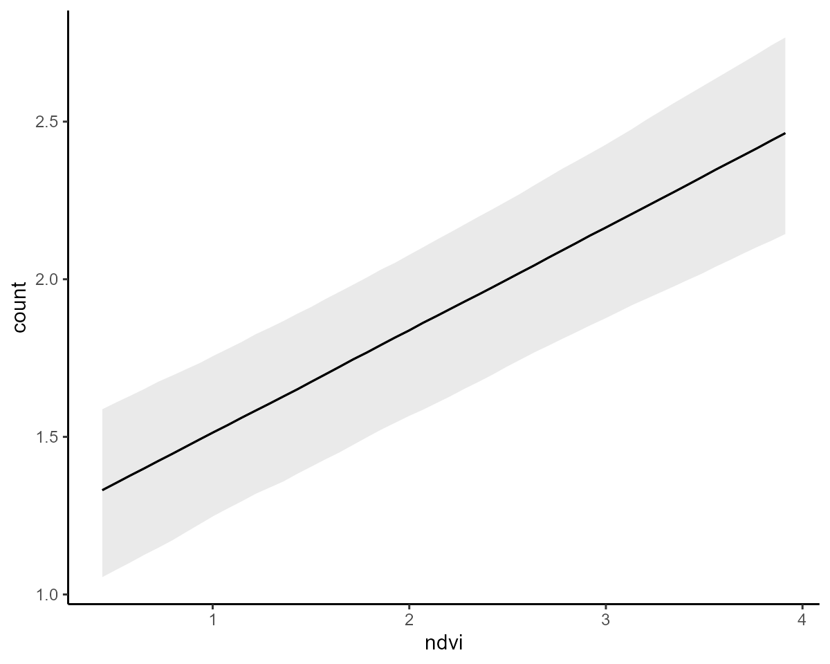
`marginaleffects` support

Given our model used a nonlinear link function (log link in this example), it can still be difficult to fully understand what relationship our model is estimating between a predictor and the response. Fortunately, the marginaleffects package makes this relatively straightforward. Objects of class mvgam can be used with marginaleffects to inspect contrasts, scenario-based predictions, conditional and marginal effects, all on the outcome scale. Here we will use the plot_predictions function from marginaleffects to inspect the conditional effect of ndvi (use ?plot_predictions for guidance on how to modify these plots):

plot_predictions(model2, 
                 condition = "ndvi",
                 # include the observed count values
                 # as points, and show rugs for the observed
                 # ndvi and count values on the axes
                 points = 0.5, rug = TRUE)

Now it is easier to get a sense of the nonlinear but positive relationship estimated between ndvi and count. Like brms, mvgam has the simple conditional_effects function to make quick and informative plots for main effects. This will likely be your go-to function for quickly understanding patterns from fitted mvgam models

plot(conditional_effects(model2)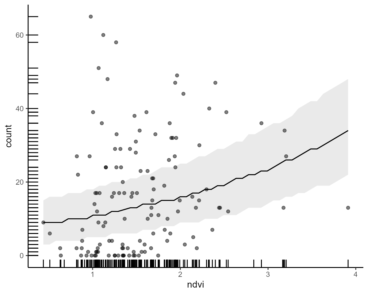, ask = FALSE)

Adding predictors as smooths

Smooth functions, using penalized splines, are a major feature of mvgam. Nonlinear splines are commonly viewed as variations of random effects in which the coefficients that control the shape of the spline are drawn from a joint, penalized distribution. This strategy is very often used in ecological time series analysis to capture smooth temporal variation in the processes we seek to study. When we construct smoothing splines, the workhorse package mgcv will calculate a set of basis functions that will collectively control the shape and complexity of the resulting spline. It is often helpful to visualize these basis functions to get a better sense of how splines work. We’ll create a set of 6 basis functions to represent possible variation in the effect of time on our outcome.In addition to constructing the basis functions, mgcv also creates a penalty matrix \(S\), which contains known coefficients that work to constrain the wiggliness of the resulting smooth function. When fitting a GAM to data, we must estimate the smoothing parameters (\(\lambda\)) that will penalize these matrices, resulting in constrained basis coefficients and smoother functions that are less likely to overfit the data. This is the key to fitting GAMs in a Bayesian framework, as we can jointly estimate the \(\lambda\)’s using informative priors to prevent overfitting and expand the complexity of models we can tackle. To see this in practice, we can now fit a model that replaces the yearly random effects with a smooth function of time. We will need a reasonably complex function (large k) to try and accommodate the temporal variation in our observations. Following some useful advice by Gavin Simpson, we will use a b-spline basis for the temporal smooth. Because we no longer have intercepts for each year, we also retain the primary intercept term in this model (there is no -1 in the formula now):

model3 <- mvgam(count ~ s(time, bs = 'bs', k = 15) + 
                  ndvi,
                family = poisson(),
                data = data_train,
                newdata = data_test)

The model can be described mathematically as follows: \[\begin{align*} \boldsymbol{count}_t & \sim \text{Poisson}(\lambda_t) \\ log(\lambda_t) & = f(\boldsymbol{time})_t + \beta_{ndvi} * \boldsymbol{ndvi}_t \\ f(\boldsymbol{time}) & = \sum_{k=1}^{K}b * \beta_{smooth} \\ \beta_{smooth} & \sim \text{MVNormal}(0, (\Omega * \lambda)^{-1}) \\ \beta_{ndvi} & \sim \text{Normal}(0, 1) \end{align*}\]

Where the smooth function \(f_{time}\) is built by summing across a set of weighted basis functions. The basis functions \((b)\) are constructed using a thin plate regression basis in mgcv. The weights \((\beta_{smooth})\) are drawn from a penalized multivariate normal distribution where the precision matrix \((\Omega\)) is multiplied by a smoothing penalty \((\lambda)\). If \(\lambda\) becomes large, this acts to squeeze the covariances among the weights \((\beta_{smooth})\), leading to a less wiggly spline. Note that sometimes there are multiple smoothing penalties that contribute to the covariance matrix, but I am only showing one here for simplicity. View the summary as before

summary(model3)
#> GAM formula:
#> count ~ s(time, bs = "bs", k = 15) + ndvi
#> 
#> Family:
#> poisson
#> 
#> Link function:
#> log
#> 
#> Trend model:
#> None
#> 
#> N series:
#> 1 
#> 
#> N timepoints:
#> 199 
#> 
#> Status:
#> Fitted using Stan 
#> 4 chains, each with iter = 1000; warmup = 500; thin = 1 
#> Total post-warmup draws = 2000
#> 
#> 
#> GAM coefficient (beta) estimates:
#>              2.5%   50%  97.5% Rhat n_eff
#> (Intercept)  2.00  2.10  2.200 1.00  1117
#> ndvi         0.26  0.33  0.400 1.00  1162
#> s(time).1   -2.20 -1.10 -0.021 1.00   577
#> s(time).2    0.37  1.30  2.300 1.01   361
#> s(time).3   -0.54  0.45  1.500 1.00   406
#> s(time).4    1.50  2.40  3.500 1.01   348
#> s(time).5   -1.20 -0.20  0.830 1.00   409
#> s(time).6   -0.64  0.36  1.500 1.00   375
#> s(time).7   -1.60 -0.54  0.490 1.00   406
#> s(time).8    0.52  1.50  2.500 1.01   362
#> s(time).9    1.10  2.00  3.100 1.00   369
#> s(time).10  -0.42  0.54  1.600 1.00   373
#> s(time).11   0.80  1.70  2.800 1.01   356
#> s(time).12   0.62  1.50  2.400 1.00   373
#> s(time).13  -1.20 -0.34  0.640 1.01   493
#> s(time).14  -7.40 -4.00 -1.100 1.01   442
#> 
#> Approximate significance of GAM smooths:
#>          edf Ref.df Chi.sq p-value    
#> s(time) 8.51     14    823  <2e-16 ***
#> ---
#> Signif. codes:  0 '***' 0.001 '**' 0.01 '*' 0.05 '.' 0.1 ' ' 1
#> 
#> Stan MCMC diagnostics:
#> n_eff / iter looks reasonable for all parameters
#> Rhat looks reasonable for all parameters
#> 0 of 2000 iterations ended with a divergence (0%)
#> 0 of 2000 iterations saturated the maximum tree depth of 12 (0%)
#> E-FMI indicated no pathological behavior
#> 
#> Samples were drawn using NUTS(diag_e) at Wed May 08 9:25:02 AM 2024.
#> For each parameter, n_eff is a crude measure of effective sample size,
#> and Rhat is the potential scale reduction factor on split MCMC chains
#> (at convergence, Rhat = 1)

The summary above now contains posterior estimates for the smoothing parameters as well as the basis coefficients for the nonlinear effect of time. We can visualize the conditional time effect using the plot function with type = 'smooths':

plot(model3, type = 'smooths')

By default this plots shows posterior empirical quantiles, but it can also be helpful to view some realizations of the underlying function (here, each line is a different potential curve drawn from the posterior of all possible curves):

plot(model3, type = 'smooths', realisations = TRUE,
     n_realisations = 30)

Derivatives of smooths

A useful question when modelling using GAMs is to identify where the function is changing most rapidly. To address this, we can plot estimated 1st derivatives of the spline:

plot(model3, type = 'smooths', derivatives = TRUE)

Here, values above >0 indicate the function was increasing at that time point, while values <0 indicate the function was declining. The most rapid declines appear to have been happening around timepoints 50 and again toward the end of the training period, for example.

Use conditional_effects again for useful plots on the outcome scale:

plot(conditional_effects(model3), ask = FALSE)

Or on the link scale:

plot(conditional_effects(model3, type = 'link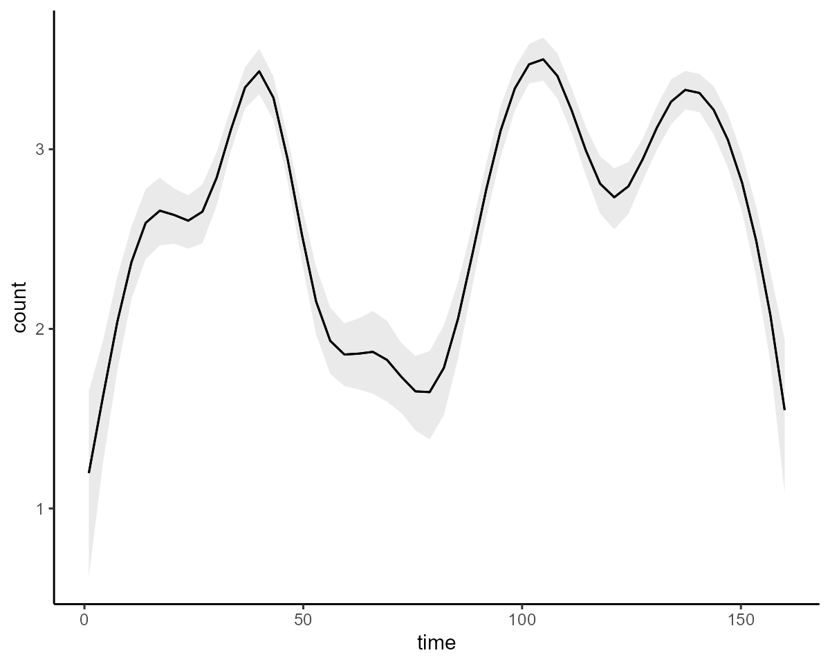'), ask = FALSE)

Inspect the underlying Stan code to gain some idea of how the spline is being penalized:

code(model3)
#> // Stan model code generated by package mvgam
#> data {
#>   int<lower=0> total_obs; // total number of observations
#>   int<lower=0> n; // number of timepoints per series
#>   int<lower=0> n_sp; // number of smoothing parameters
#>   int<lower=0> n_series; // number of series
#>   int<lower=0> num_basis; // total number of basis coefficients
#>   vector[num_basis] zero; // prior locations for basis coefficients
#>   matrix[total_obs, num_basis] X; // mgcv GAM design matrix
#>   array[n, n_series] int<lower=0> ytimes; // time-ordered matrix (which col in X belongs to each [time, series] observation?)
#>   matrix[14, 28] S1; // mgcv smooth penalty matrix S1
#>   int<lower=0> n_nonmissing; // number of nonmissing observations
#>   array[n_nonmissing] int<lower=0> flat_ys; // flattened nonmissing observations
#>   matrix[n_nonmissing, num_basis] flat_xs; // X values for nonmissing observations
#>   array[n_nonmissing] int<lower=0> obs_ind; // indices of nonmissing observations
#> }
#> parameters {
#>   // raw basis coefficients
#>   vector[num_basis] b_raw;
#>   
#>   // smoothing parameters
#>   vector<lower=0>[n_sp] lambda;
#> }
#> transformed parameters {
#>   // basis coefficients
#>   vector[num_basis] b;
#>   b[1 : num_basis] = b_raw[1 : num_basis];
#> }
#> model {
#>   // prior for (Intercept)...
#>   b_raw[1] ~ student_t(3, 2.6, 2.5);
#>   
#>   // prior for ndvi...
#>   b_raw[2] ~ student_t(3, 0, 2);
#>   
#>   // prior for s(time)...
#>   b_raw[3 : 16] ~ multi_normal_prec(zero[3 : 16],
#>                                     S1[1 : 14, 1 : 14] * lambda[1]
#>                                     + S1[1 : 14, 15 : 28] * lambda[2]);
#>   
#>   // priors for smoothing parameters
#>   lambda ~ normal(5, 30);
#>   {
#>     // likelihood functions
#>     flat_ys ~ poisson_log_glm(flat_xs, 0.0, b);
#>   }
#> }
#> generated quantities {
#>   vector[total_obs] eta;
#>   matrix[n, n_series] mus;
#>   vector[n_sp] rho;
#>   array[n, n_series] int ypred;
#>   rho = log(lambda);
#>   
#>   // posterior predictions
#>   eta = X * b;
#>   for (s in 1 : n_series) {
#>     mus[1 : n, s] = eta[ytimes[1 : n, s]];
#>     ypred[1 : n, s] = poisson_log_rng(mus[1 : n, s]);
#>   }
#> }

The line below // prior for s(time)... shows how the spline basis coefficients are drawn from a zero-centred multivariate normal distribution. The precision matrix \(S\) is penalized by two different smoothing parameters (the \(\lambda\)’s) to enforce smoothness and reduce overfitting

Latent dynamics in `mvgam`

Forecasts from the above model are not ideal:

plot(model3, type = 'forecast', newdata = data_test)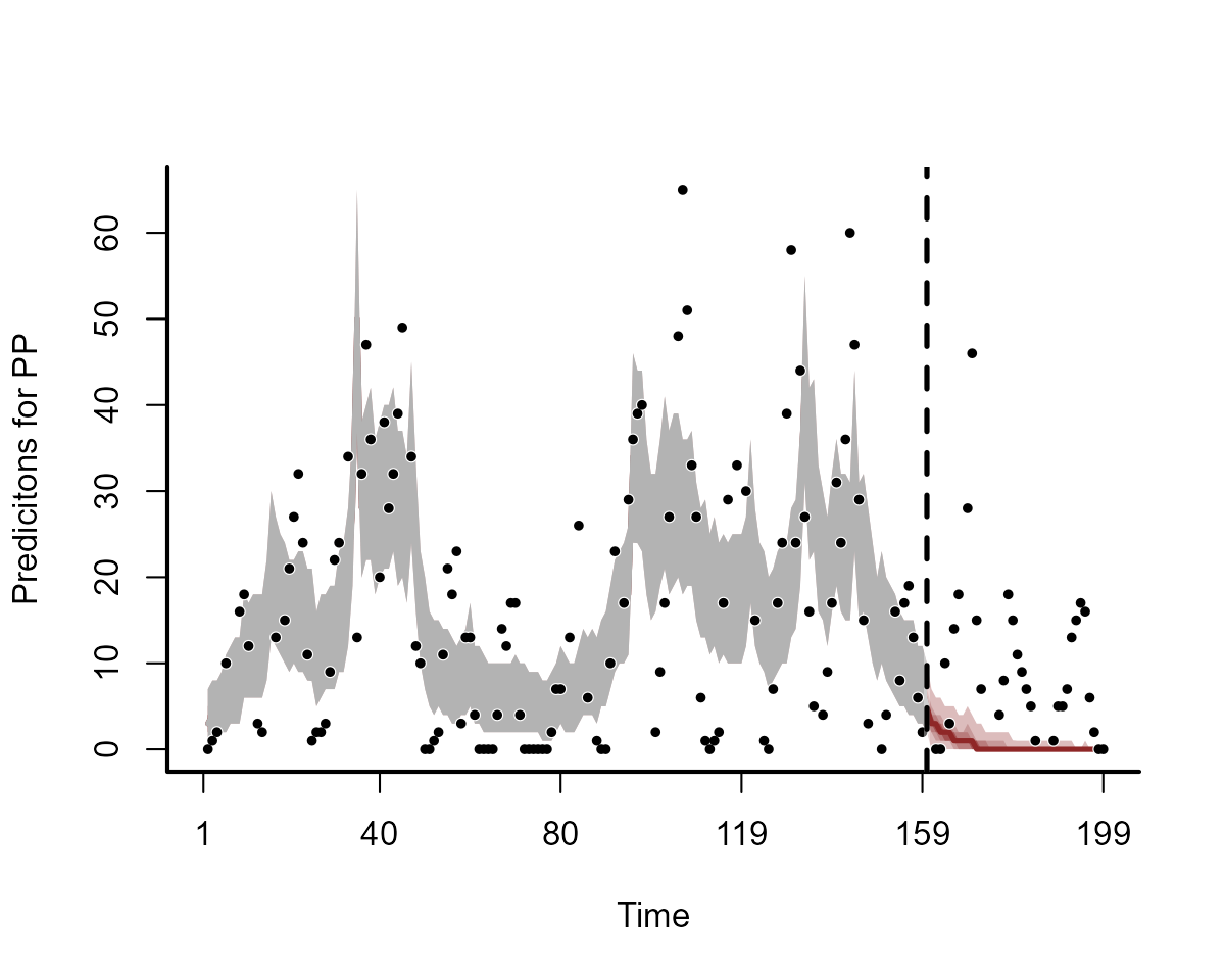
#> Out of sample DRPS:
#> 286.045292

Why is this happening? The forecasts are driven almost entirely by variation in the temporal spline, which is extrapolating linearly forever beyond the edge of the training data. Any slight wiggles near the end of the training set will result in wildly different forecasts. To visualize this, we can plot the extrapolated temporal functions into the out-of-sample test set for the two models. Here are the extrapolated functions for the first model, with 15 basis functions:

plot_mvgam_smooth(model3, smooth = 's(time)',
                  # feed newdata to the plot function to generate
                  # predictions of the temporal smooth to the end of the 
                  # testing period
                  newdata = data.frame(time = 1:max(data_test$time),
                                       ndvi = 0))
abline(v = max(data_train$time), lty = 'dashed', lwd = 2)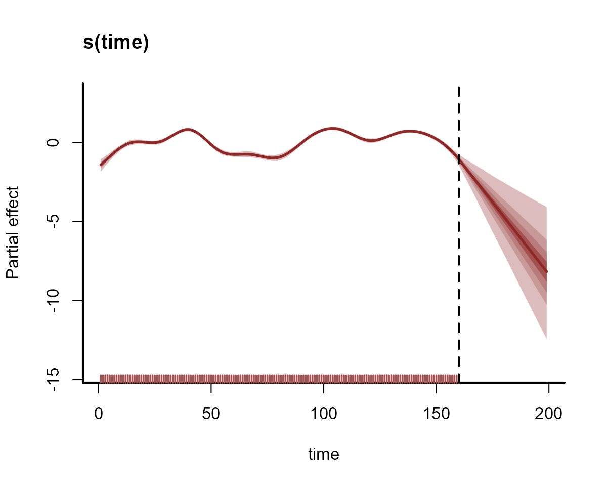

This model is not doing well. Clearly we need to somehow account for the strong temporal autocorrelation when modelling these data without using a smooth function of time. Now onto another prominent feature of mvgam: the ability to include (possibly latent) autocorrelated residuals in regression models. To do so, we use the trend_model argument (see ?mvgam_trends for details of different dynamic trend models that are supported). This model will use a separate sub-model for latent residuals that evolve as an AR1 process (i.e. the error in the current time point is a function of the error in the previous time point, plus some stochastic noise). We also include a smooth function of ndvi in this model, rather than the parametric term that was used above, to showcase that mvgam can include combinations of smooths and dynamic components:

model4 <- mvgam(count ~ s(ndvi, k = 6),
                family = poisson(),
                data = data_train,
                newdata = data_test,
                trend_model = 'AR1')

The model can be described mathematically as follows: \[\begin{align*} \boldsymbol{count}_t & \sim \text{Poisson}(\lambda_t) \\ log(\lambda_t) & = f(\boldsymbol{ndvi})_t + z_t \\ z_t & \sim \text{Normal}(ar1 * z_{t-1}, \sigma_{error}) \\ ar1 & \sim \text{Normal}(0, 1)[-1, 1] \\ \sigma_{error} & \sim \text{Exponential}(2) \\ f(\boldsymbol{ndvi}) & = \sum_{k=1}^{K}b * \beta_{smooth} \\ \beta_{smooth} & \sim \text{MVNormal}(0, (\Omega * \lambda)^{-1}) \end{align*}\]

Here the term \(z_t\) captures autocorrelated latent residuals, which are modelled using an AR1 process. You can also notice that this model is estimating autocorrelated errors for the full time period, even though some of these time points have missing observations. This is useful for getting more realistic estimates of the residual autocorrelation parameters. Summarise the model to see how it now returns posterior summaries for the latent AR1 process:

summary(model4)
#> GAM formula:
#> count ~ s(ndvi, k = 6)
#> 
#> Family:
#> poisson
#> 
#> Link function:
#> log
#> 
#> Trend model:
#> AR1
#> 
#> N series:
#> 1 
#> 
#> N timepoints:
#> 199 
#> 
#> Status:
#> Fitted using Stan 
#> 4 chains, each with iter = 1000; warmup = 500; thin = 1 
#> Total post-warmup draws = 2000
#> 
#> 
#> GAM coefficient (beta) estimates:
#>               2.5%      50% 97.5% Rhat n_eff
#> (Intercept)  0.810  1.90000 2.500 1.12    27
#> s(ndvi).1   -0.075  0.01200 0.180 1.00   386
#> s(ndvi).2   -0.150  0.01900 0.380 1.01   357
#> s(ndvi).3   -0.064 -0.00074 0.056 1.00   846
#> s(ndvi).4   -0.250  0.13000 1.600 1.01   201
#> s(ndvi).5   -0.098  0.15000 0.340 1.01   372
#> 
#> Approximate significance of GAM smooths:
#>          edf Ref.df Chi.sq p-value  
#> s(ndvi) 3.13      5   83.8    0.07 .
#> ---
#> Signif. codes:  0 '***' 0.001 '**' 0.01 '*' 0.05 '.' 0.1 ' ' 1
#> 
#> Latent trend parameter AR estimates:
#>          2.5%  50% 97.5% Rhat n_eff
#> ar1[1]   0.70 0.81  0.94 1.03    90
#> sigma[1] 0.68 0.80  0.96 1.00   465
#> 
#> Stan MCMC diagnostics:
#> n_eff / iter looks reasonable for all parameters
#> Rhats above 1.05 found for 96 parameters
#>  *Diagnose further to investigate why the chains have not mixed
#> 0 of 2000 iterations ended with a divergence (0%)
#> 0 of 2000 iterations saturated the maximum tree depth of 12 (0%)
#> E-FMI indicated no pathological behavior
#> 
#> Samples were drawn using NUTS(diag_e) at Wed May 08 9:26:04 AM 2024.
#> For each parameter, n_eff is a crude measure of effective sample size,
#> and Rhat is the potential scale reduction factor on split MCMC chains
#> (at convergence, Rhat = 1)

View conditional smooths for the ndvi effect:

plot_predictions(model4, 
                 condition = "ndvi",
                 points = 0.5, rug = TRUE)

View posterior hindcasts / forecasts and compare against the out of sample test data

plot(model4, type = 'forecast', newdata = data_test)
#> Out of sample DRPS:
#> 152.86676175

The trend is evolving as an AR1 process, which we can also view:

plot(model4, type = 'trend', newdata = data_test)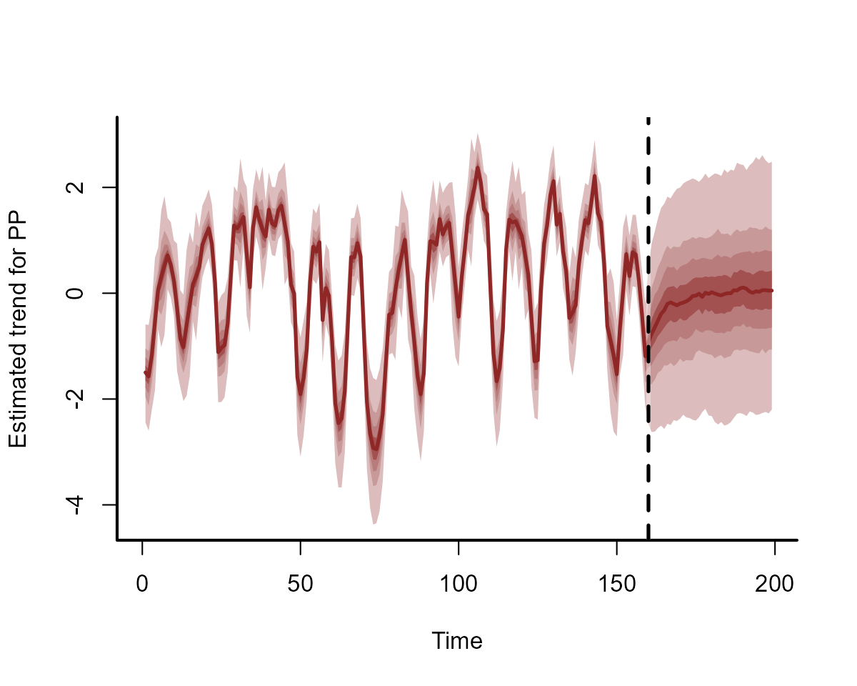

In-sample model performance can be interrogated using leave-one-out cross-validation utilities from the loo package (a higher value is preferred for this metric):

loo_compare(model3, model4)
#> Warning: Some Pareto k diagnostic values are too high. See help('pareto-k-diagnostic') for details.

#> Warning: Some Pareto k diagnostic values are too high. See help('pareto-k-diagnostic') for details.
#>        elpd_diff se_diff
#> model4    0.0       0.0 
#> model3 -560.4      66.4

The higher estimated log predictive density (ELPD) value for the dynamic model suggests it provides a better fit to the in-sample data.

Though it should be obvious that this model provides better forecasts, we can quantify forecast performance for models 3 and 4 using the forecast and score functions. Here we will compare models based on their Discrete Ranked Probability Scores (a lower value is preferred for this metric)

fc_mod3 <- forecast(model3)
fc_mod4 <- forecast(model4)
score_mod3 <- score(fc_mod3, score = 'drps')
score_mod4 <- score(fc_mod4, score = 'drps')
sum(score_mod4$PP$score, na.rm = TRUE) - sum(score_mod3$PP$score, na.rm = TRUE)
#> [1] -133.1785

A strongly negative value here suggests the score for the dynamic model (model 4) is much smaller than the score for the model with a smooth function of time (model 3)

Interested in contributing?

I’m actively seeking PhD students and other researchers to work in the areas of ecological forecasting, multivariate model evaluation and development of mvgam. Please reach out if you are interested (n.clark’at’uq.edu.au)

Nicholas J Clark

2024-05-08

Dynamic GAMs

Supported observation families

Supported temporal dynamic processes

Independent Random Walks

Multivariate Random Walks

Autoregressive processes

Vector Autoregressive processes

Gaussian Processes

Piecewise logistic and linear trends

Continuous time AR(1) processes

Regression formulae

Example time series data

Manipulating data for modelling

GLMs with temporal random effects

Plotting effects and residuals

`bayesplot` support

Automatic forecasting for new data

Adding predictors as “fixed” effects

`marginaleffects` support

Adding predictors as smooths

Derivatives of smooths

Latent dynamics in `mvgam`

Interested in contributing?

Overview of the mvgam package

Nicholas J Clark

2024-05-08

Dynamic GAMs

Supported observation families

Supported temporal dynamic processes

Independent Random Walks

Multivariate Random Walks

Autoregressive processes

Vector Autoregressive processes

Gaussian Processes

Piecewise logistic and linear trends

Continuous time AR(1) processes

Regression formulae

Example time series data

Manipulating data for modelling

GLMs with temporal random effects

Plotting effects and residuals

bayesplot support

Automatic forecasting for new data

Adding predictors as “fixed” effects

marginaleffects support

Adding predictors as smooths

Derivatives of smooths

Latent dynamics in mvgam

Interested in contributing?

`bayesplot` support

`marginaleffects` support

Latent dynamics in `mvgam`