Predict from a fitted mvgam model

Usage

# S3 method for mvgam
predict(
  object,
  newdata,
  data_test,
  type = "link",
  process_error = FALSE,
  summary = TRUE,
  robust = FALSE,
  probs = c(0.025, 0.975),
  ...
)

Arguments

object: list object of class mvgam or jsdgam. See mvgam()
newdata: Optional dataframe or list of test data containing the same variables that were included in the original data used to fit the model. If not supplied, predictions are generated for the original observations used for the model fit.
data_test: Deprecated. Still works in place of newdata but users are recommended to use newdata instead for more seamless integration into R workflows
type: When this has the value link (default) the linear predictor is calculated on the link scale. If expected is used, predictions reflect the expectation of the response (the mean) but ignore uncertainty in the observation process. When response is used, the predictions take uncertainty in the observation process into account to return predictions on the outcome scale. When variance is used, the variance of the response with respect to the mean (mean-variance relationship) is returned. When type = "terms", each component of the linear predictor is returned separately in the form of a list (possibly with standard errors, if summary = TRUE): this includes parametric model components, followed by each smooth component, but excludes any offset and any intercept. Two special cases are also allowed: type latent_N will return the estimated latent abundances from an N-mixture distribution, while type detection will return the estimated detection probability from an N-mixture distribution
process_error: Logical. If TRUE and a dynamic trend model was fit, expected uncertainty in the process model is accounted for by using draws from a stationary, zero-centred multivariate Normal distribution using any estimated process variance-covariance parameters. If FALSE, uncertainty in the latent trend component is ignored when calculating predictions
summary: Should summary statistics be returned instead of the raw values? Default is TRUE..
robust: If FALSE (the default) the mean is used as the measure of central tendency and the standard deviation as the measure of variability. If TRUE, the median and the median absolute deviation (MAD) are applied instead. Only used if summary is TRUE.
probs: The percentiles to be computed by the quantile function. Only used if summary is TRUE.
...: Ignored

Value

Predicted values on the appropriate scale. If summary = FALSE and type != "terms", the output is a matrix of dimension n_draw x n_observations

containing predicted values for each posterior draw in object.

If summary = TRUE and type != "terms", the output is an n_observations x E

matrix. The number of summary statistics E is equal to 2 + length(probs): The Estimate column contains point estimates (either mean or median depending on argument robust), while the Est.Error column contains uncertainty estimates (either standard deviation or median absolute deviation depending on argument robust). The remaining columns starting with Q contain quantile estimates as specified via argument probs.

If type = "terms" and summary = FALSE, the output is a named list

containing a separate slot for each effect, with the effects returned as matrices of dimension n_draw x 1. If summary = TRUE, the output resembles that from predict.gam when using the call predict.gam(object, type = "terms", se.fit = TRUE), where mean contributions from each effect are returned in matrix form while standard errors (representing the interval: (max(probs) - min(probs)) / 2) are returned in a separate matrix

Details

Note that if your model included a latent temporal trend (i.e. if you used something other than "None" for the trend_model argument), the predictions returned by this function will ignore autocorrelation coefficients or GP length scale coefficients by assuming the process is stationary. This approach is similar to how predictions are computed from other types of regression models that can include correlated residuals, ultimately treating the temporal dynamics as random effect nuisance parameters. The predict function is therefore more suited to scenario-based posterior simulation from the GAM components of a mvgam model, while the hindcast / forecast functions hindcast.mvgam() and forecast.mvgam() are better suited to generate predictions that respect the temporal dynamics of estimated latent trends at the actual time points supplied in data and newdata.

Author

Nicholas J Clark

Examples

# \donttest{
# Simulate 4 time series with hierarchical seasonality
# and independent AR1 dynamic processes
set.seed(123)
simdat <- sim_mvgam(
seasonality = 'hierarchical',
prop_trend = 0.75,
trend_model = AR(),
family = gaussian()
)
set.seed(111)
# Fit a model with shared seasonality
# and AR(1) dynamics
mod1 <- mvgam(
y ~ s(season, bs = 'cc', k = 6),
data = simdat$data_train,
family = gaussian(),
trend_model = AR(),
noncentred = TRUE,
chains = 2,
silent = 2
)

# Generate predictions against observed data
preds <- predict(
mod1,
summary = TRUE
)
head(preds)
#>        Estimate  Est.Error       Q2.5      Q97.5
#> [1,] -0.6322340 0.09297519 -0.8128206 -0.4453673
#> [2,] -0.6322340 0.09297519 -0.8128206 -0.4453673
#> [3,] -0.6322340 0.09297519 -0.8128206 -0.4453673
#> [4,] -0.6978479 0.09575656 -0.8851124 -0.5058719
#> [5,] -0.6978479 0.09575656 -0.8851124 -0.5058719
#> [6,] -0.6978479 0.09575656 -0.8851124 -0.5058719

# Generate predictions against test data
preds <- predict(
mod1,
newdata = simdat$data_test,
summary = TRUE
)
head(preds)
#>        Estimate Est.Error       Q2.5      Q97.5
#> [1,] -0.6209420 0.1107312 -0.8243132 -0.3948167
#> [2,] -0.6209420 0.1107312 -0.8243132 -0.3948167
#> [3,] -0.6209420 0.1107312 -0.8243132 -0.3948167
#> [4,] -0.4739291 0.1166200 -0.6863414 -0.2293952
#> [5,] -0.4739291 0.1166200 -0.6863414 -0.2293952
#> [6,] -0.4739291 0.1166200 -0.6863414 -0.2293952

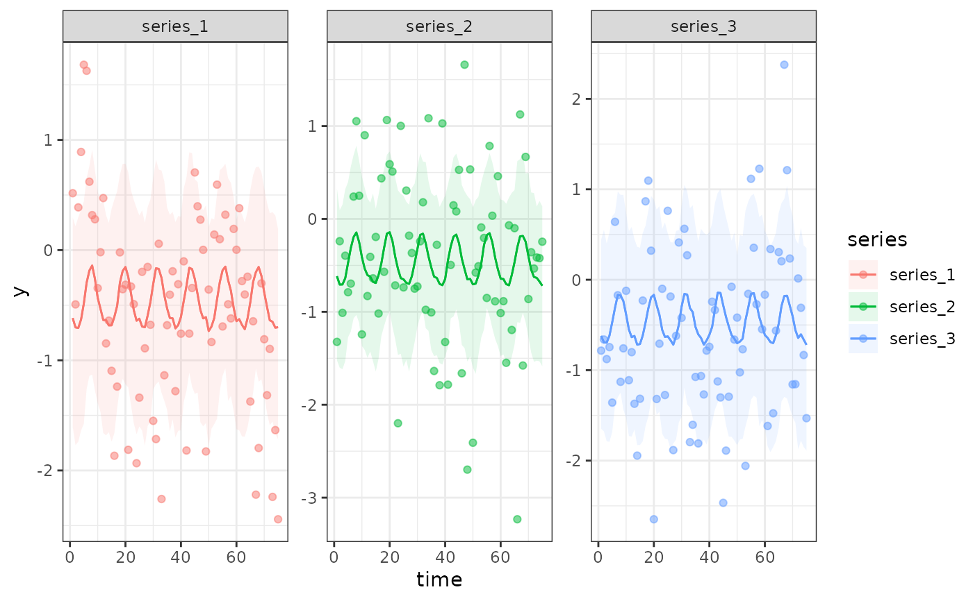
# Use plot_predictions(), which relies on predict()
# to more easily see how the latent AR(1) dynamics are
# being ignored when using predict()
plot_predictions(
mod1,
by = c('time', 'series', 'series'),
points = 0.5
)


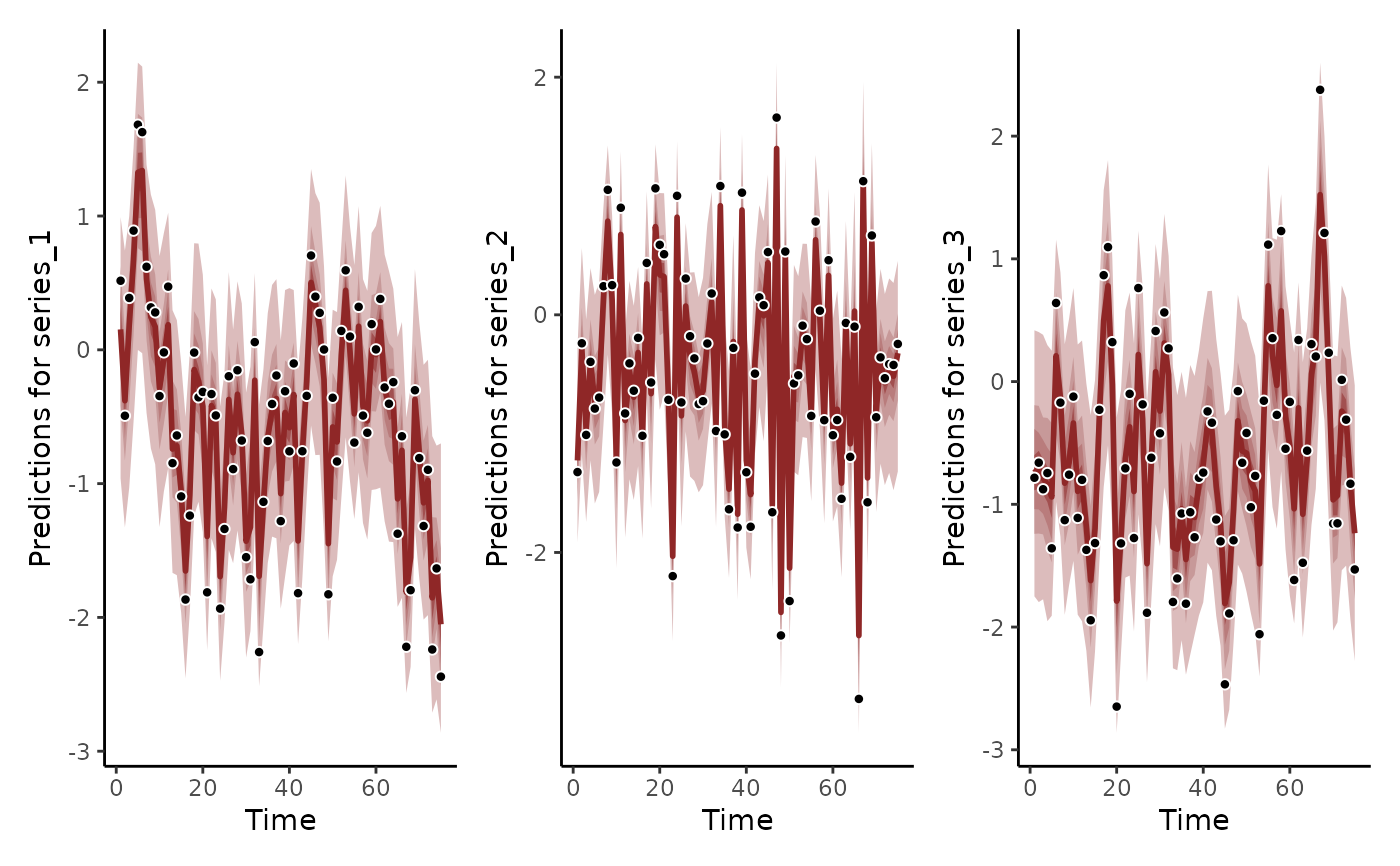
# Using the hindcast() function will give a more accurate
# representation of how the AR(1) processes were estimated to give
# accurate predictions to the in-sample training data
hc <- hindcast(mod1)
plot(hc) +
plot(hc, series = 2) +
plot(hc, series = 3)
#> No non-missing values in test_observations; cannot calculate forecast score
#> No non-missing values in test_observations; cannot calculate forecast score
#> No non-missing values in test_observations; cannot calculate forecast score

# }