Skip to contents

This function takes a fitted mvgam object and produces plots of smooth functions, forecasts, trends and uncertainty components

Usage

# S3 method for mvgam
plot(
  x,
  type = "residuals",
  series = 1,
  residuals = FALSE,
  newdata,
  data_test,
  trend_effects = FALSE,
  ...
)

Arguments

x

list object returned from mvgam. See mvgam()

type

character specifying which type of plot to return. Options are: series, residuals, smooths, re (random effect smooths), pterms (parametric effects), forecast, trend, uncertainty, factors

series

integer specifying which series in the set is to be plotted. This is ignored if type == 're'

residuals

logical. If TRUE and type = 'smooths', posterior quantiles of partial residuals are added to plots of 1-D smooths as a series of ribbon rectangles. Partial residuals for a smooth term are the median Dunn-Smyth residuals that would be obtained by dropping the term concerned from the model, while leaving all other estimates fixed (i.e. the estimates for the term plus the original median Dunn-Smyth residuals). Note that because mvgam works with Dunn-Smyth residuals and not working residuals, which are used by mgcv, the magnitudes of partial residuals will be different to what you would expect from plot.gam. Interpretation is similar though, as these partial residuals should be evenly scattered around the smooth function if the function is well estimated

newdata

Optional dataframe or list of test data containing at least 'series' and 'time' in addition to any other variables included in the linear predictor of the original formula. This argument is optional when plotting out of sample forecast period observations (when type = forecast) and required when plotting uncertainty components (type = uncertainty).

data_test

Deprecated. Still works in place of newdata but users are recommended to use newdata instead for more seamless integration into R workflows

trend_effects

logical. If TRUE and a trend_formula was used in model fitting, terms from the trend (i.e. process) model will be plotted

...

Additional arguments for each individual plotting function.

Value

A base R plot or set of plots

Details

These plots are useful for getting an overview of the fitted model and its estimated random effects or smooth functions, but the individual plotting functions and the functions from the marginaleffects and gratia packages offer far more more customisation.

Author

Nicholas J Clark

Examples

# \donttest{
# Simulate some time series
dat <- sim_mvgam(T = 80, n_series = 3)

# Fit a basic model
mod <- mvgam(y ~ s(season, bs = 'cc') + s(series, bs = 're'),
            data = dat$data_train,
            trend_model = RW(),
            chains = 2)
#> Your model may benefit from using "noncentred = TRUE"
#> Compiling Stan program using cmdstanr
#> 
#> In file included from stan/lib/stan_math/stan/math/prim/prob/von_mises_lccdf.hpp:5,
#>                  from stan/lib/stan_math/stan/math/prim/prob/von_mises_ccdf_log.hpp:4,
#>                  from stan/lib/stan_math/stan/math/prim/prob.hpp:359,
#>                  from stan/lib/stan_math/stan/math/prim.hpp:16,
#>                  from stan/lib/stan_math/stan/math/rev.hpp:16,
#>                  from stan/lib/stan_math/stan/math.hpp:19,
#>                  from stan/src/stan/model/model_header.hpp:4,
#>                  from C:/Users/uqnclar2/AppData/Local/Temp/RtmpuihtV8/model-49f827f5212f.hpp:2:
#> stan/lib/stan_math/stan/math/prim/prob/von_mises_cdf.hpp: In function 'stan::return_type_t<T_x, T_sigma, T_l> stan::math::von_mises_cdf(const T_x&, const T_mu&, const T_k&)':
#> stan/lib/stan_math/stan/math/prim/prob/von_mises_cdf.hpp:194: note: '-Wmisleading-indentation' is disabled from this point onwards, since column-tracking was disabled due to the size of the code/headers
#>   194 |       if (cdf_n < 0.0)
#>       | 
#> stan/lib/stan_math/stan/math/prim/prob/von_mises_cdf.hpp:194: note: adding '-flarge-source-files' will allow for more column-tracking support, at the expense of compilation time and memory
#> Start sampling
#> Running MCMC with 2 parallel chains...
#> 
#> Chain 1 Iteration:   1 / 1000 [  0%]  (Warmup) 
#> Chain 2 Iteration:   1 / 1000 [  0%]  (Warmup) 
#> Chain 2 Iteration: 100 / 1000 [ 10%]  (Warmup) 
#> Chain 1 Iteration: 100 / 1000 [ 10%]  (Warmup) 
#> Chain 1 Iteration: 200 / 1000 [ 20%]  (Warmup) 
#> Chain 2 Iteration: 200 / 1000 [ 20%]  (Warmup) 
#> Chain 1 Iteration: 300 / 1000 [ 30%]  (Warmup) 
#> Chain 2 Iteration: 300 / 1000 [ 30%]  (Warmup) 
#> Chain 1 Iteration: 400 / 1000 [ 40%]  (Warmup) 
#> Chain 2 Iteration: 400 / 1000 [ 40%]  (Warmup) 
#> Chain 1 Iteration: 500 / 1000 [ 50%]  (Warmup) 
#> Chain 1 Iteration: 501 / 1000 [ 50%]  (Sampling) 
#> Chain 2 Iteration: 500 / 1000 [ 50%]  (Warmup) 
#> Chain 2 Iteration: 501 / 1000 [ 50%]  (Sampling) 
#> Chain 1 Iteration: 600 / 1000 [ 60%]  (Sampling) 
#> Chain 2 Iteration: 600 / 1000 [ 60%]  (Sampling) 
#> Chain 2 Iteration: 700 / 1000 [ 70%]  (Sampling) 
#> Chain 1 Iteration: 700 / 1000 [ 70%]  (Sampling) 
#> Chain 2 Iteration: 800 / 1000 [ 80%]  (Sampling) 
#> Chain 1 Iteration: 800 / 1000 [ 80%]  (Sampling) 
#> Chain 2 Iteration: 900 / 1000 [ 90%]  (Sampling) 
#> Chain 2 Iteration: 1000 / 1000 [100%]  (Sampling) 
#> Chain 2 finished in 6.5 seconds.
#> Chain 1 Iteration: 900 / 1000 [ 90%]  (Sampling) 
#> Chain 1 Iteration: 1000 / 1000 [100%]  (Sampling) 
#> Chain 1 finished in 7.5 seconds.
#> 
#> Both chains finished successfully.
#> Mean chain execution time: 7.0 seconds.
#> Total execution time: 7.6 seconds.
#> 

# Plot predictions and residuals for each series
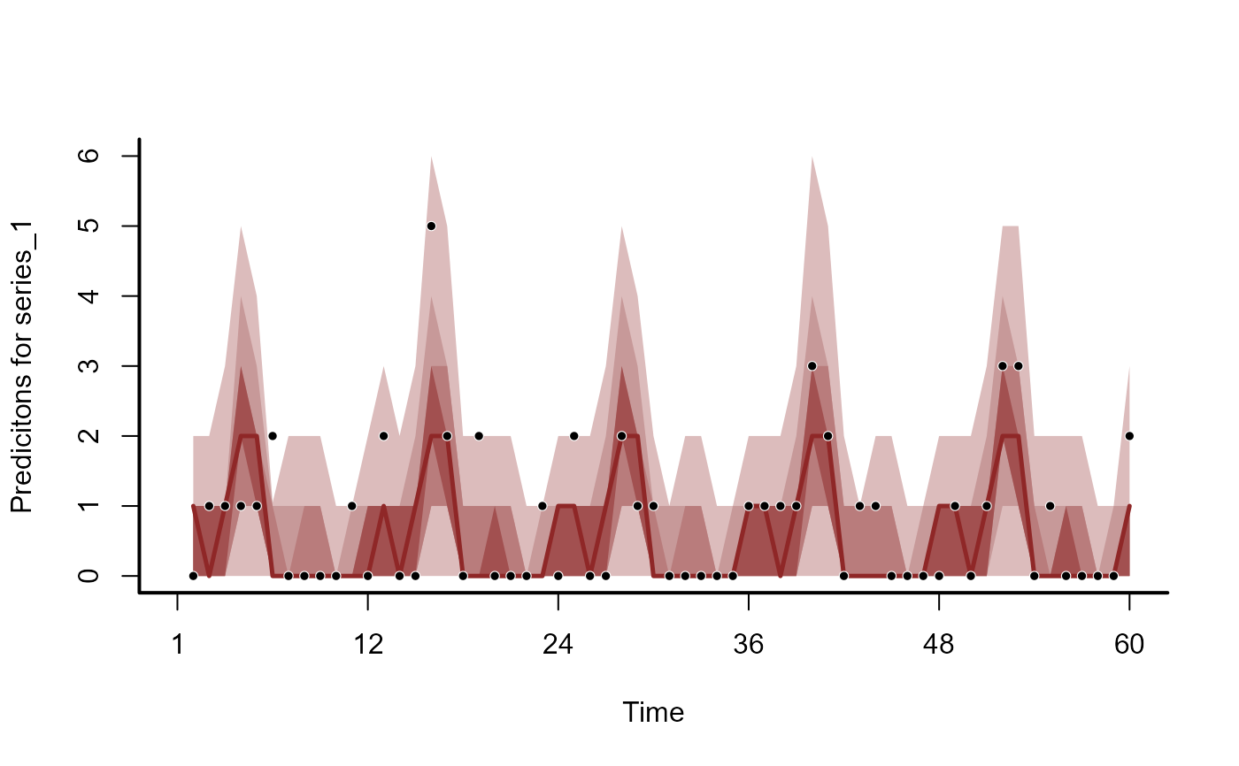
plot(mod, type = 'forecast', series = 1)
plot(mod, type = 'forecast', series = 2)
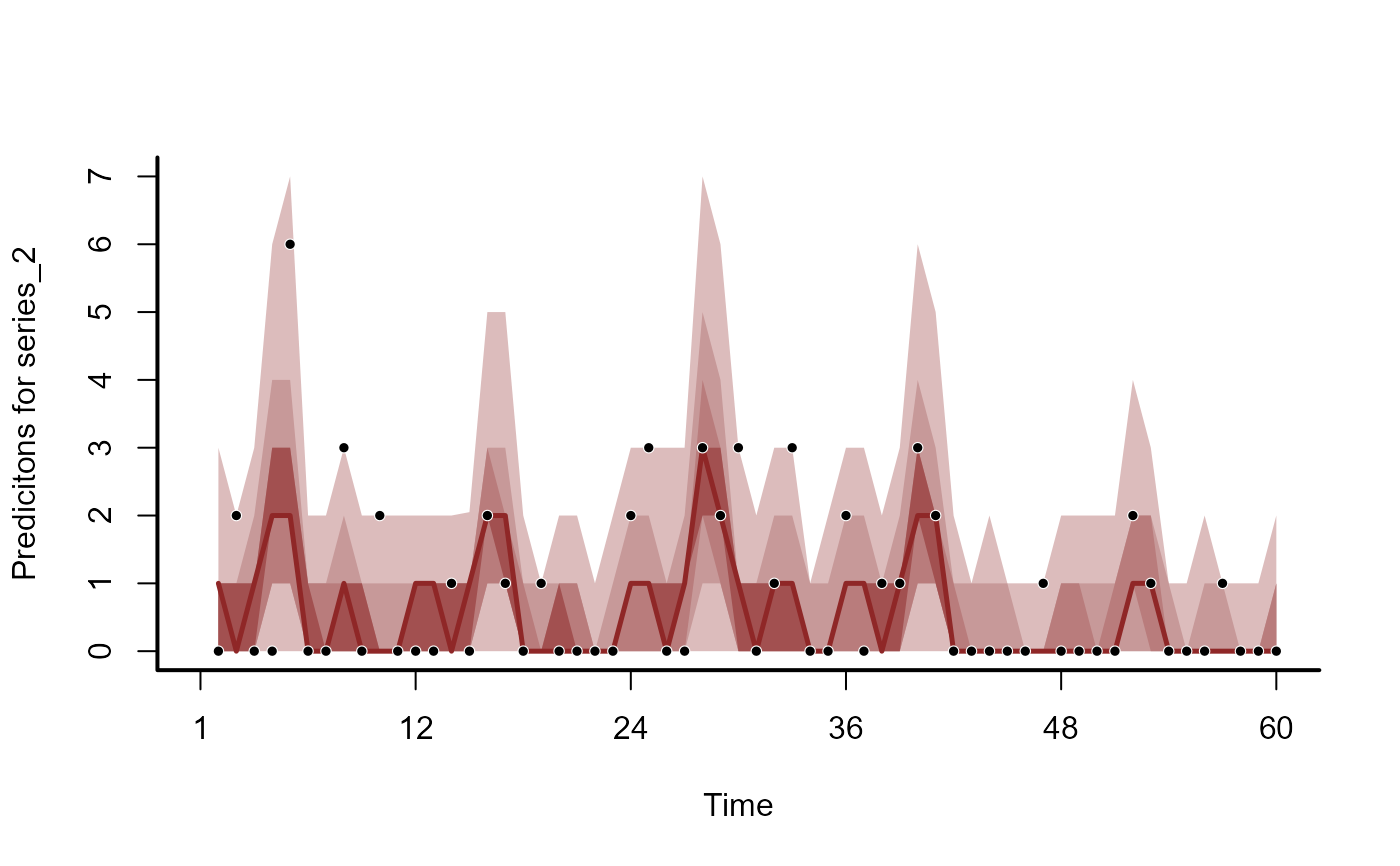
plot(mod, type = 'forecast', series = 3)
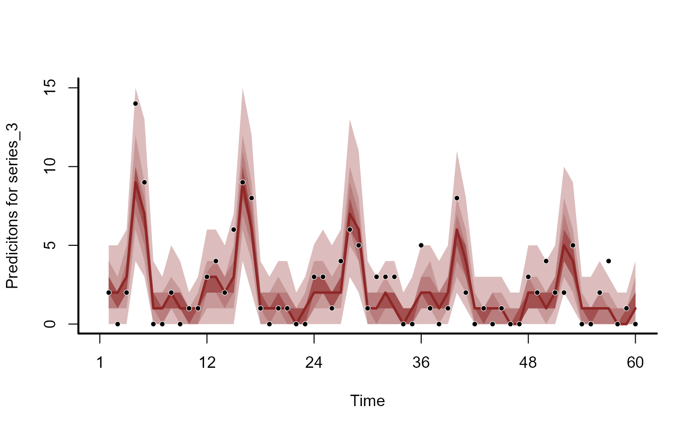
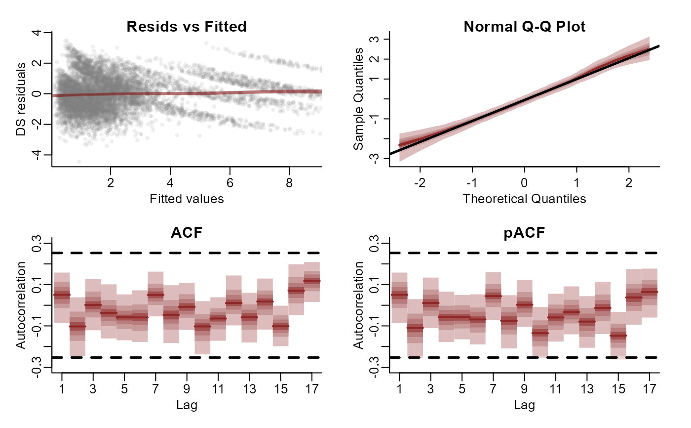
plot(mod, type = 'residuals', series = 1)
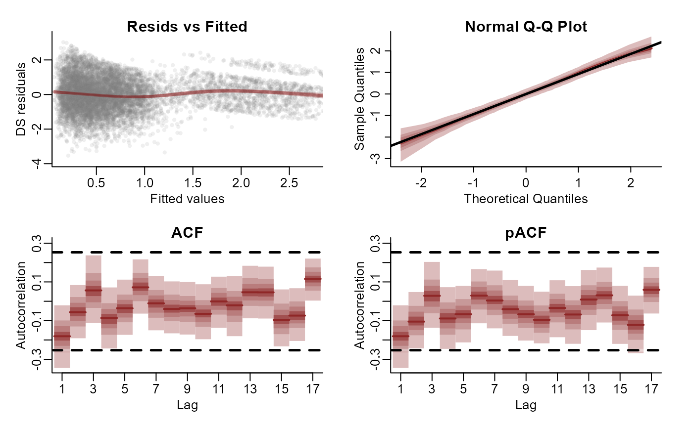
plot(mod, type = 'residuals', series = 2)
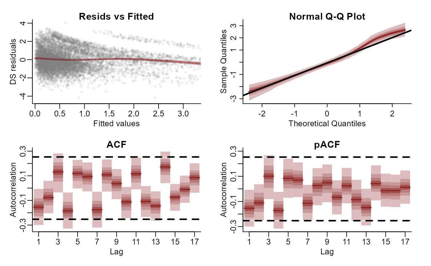
plot(mod, type = 'residuals', series = 3)

# Plot model effects
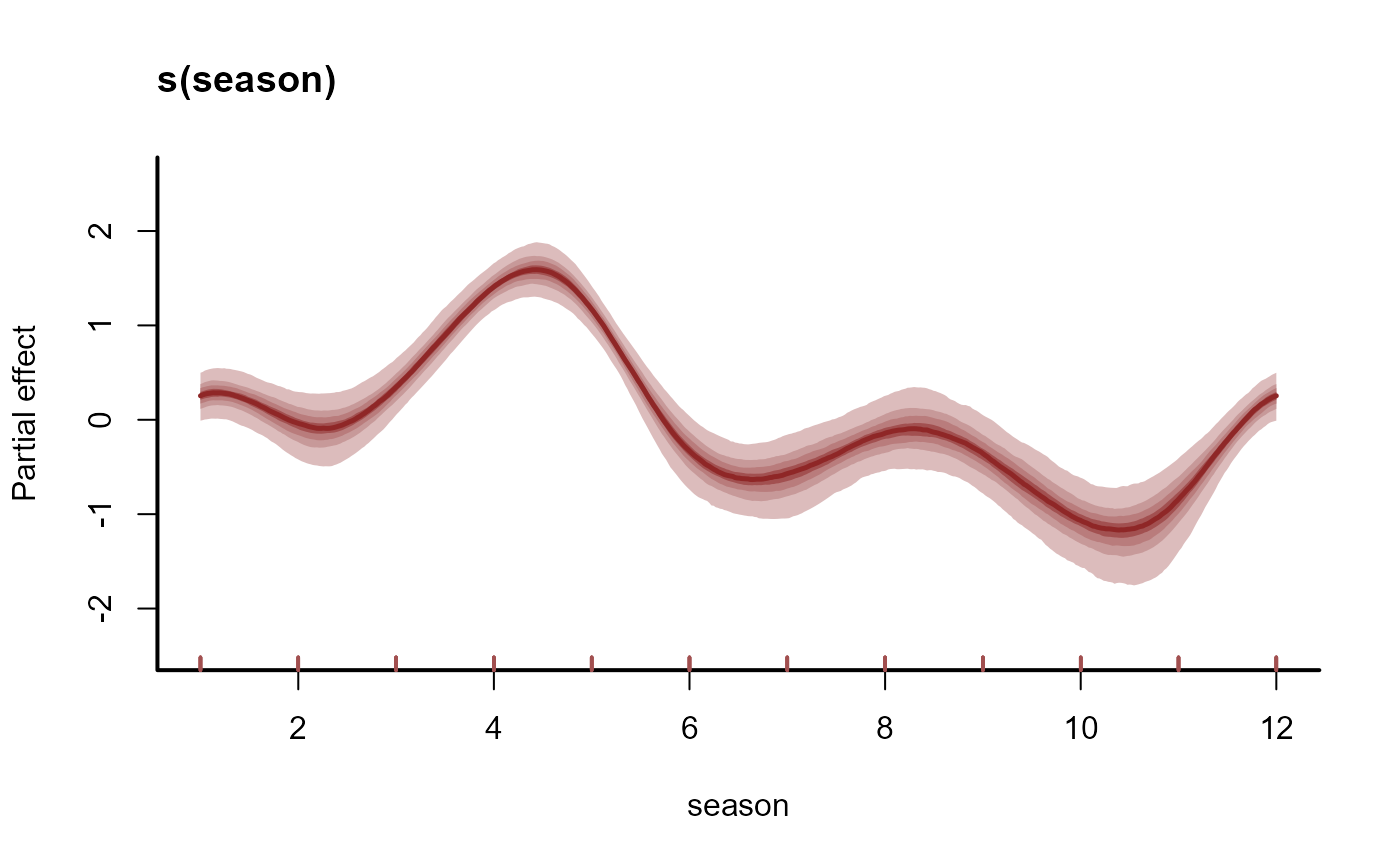
plot(mod, type = 'smooths')
plot(mod, type = 're')


# More flexible plots with 'marginaleffects' utilities
library(marginaleffects)
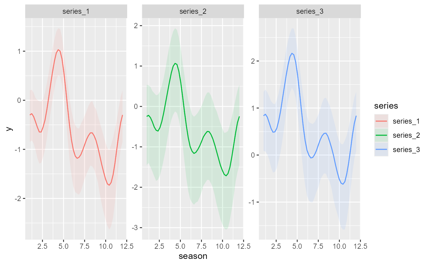
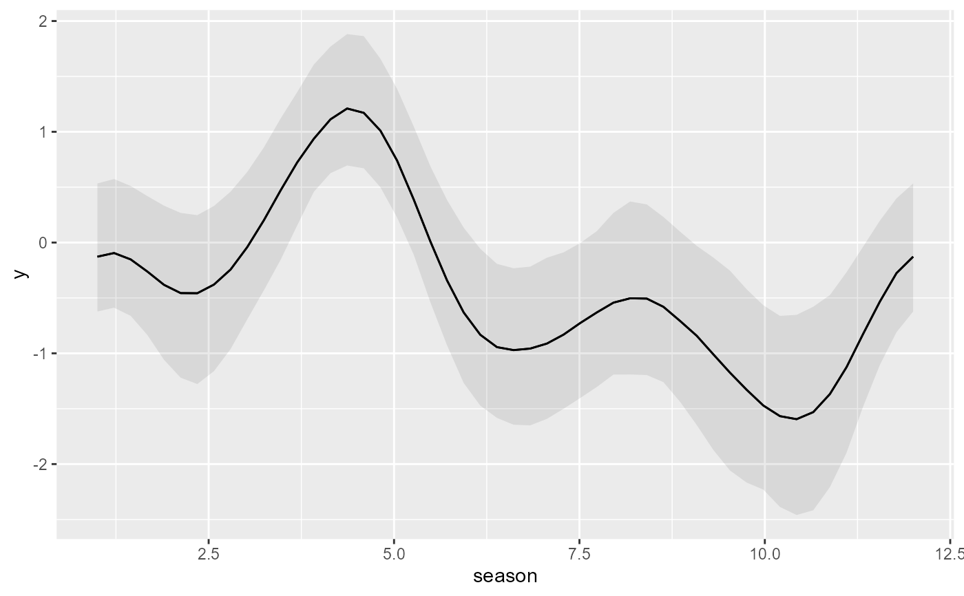
plot_predictions(mod, condition = 'season', type = 'link')

plot_predictions(mod,
                condition = c('season', 'series', 'series'),
                type = 'link')

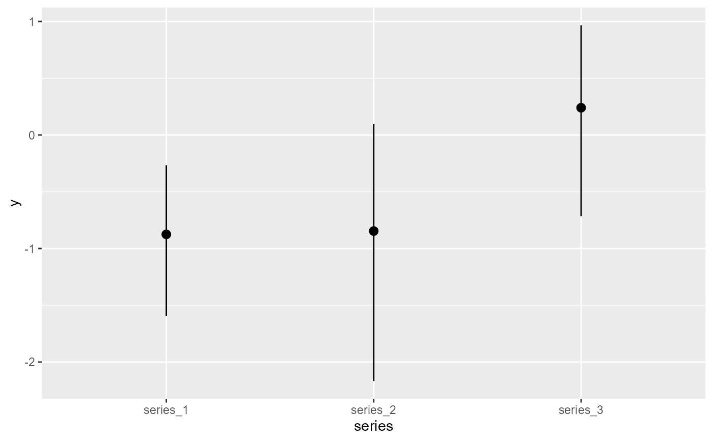
plot_predictions(mod, condition = 'series', type = 'link')


# When using a State-Space model with predictors on the process
# model, set trend_effects = TRUE to visualise process effects
mod <- mvgam(y ~ -1,
            trend_formula = ~ s(season, bs = 'cc'),
            data = dat$data_train,
            trend_model = RW(),
            chains = 2)
#> Your model may benefit from using "noncentred = TRUE"
#> Compiling Stan program using cmdstanr
#> 
#> In file included from stan/lib/stan_math/stan/math/prim/prob/von_mises_lccdf.hpp:5,
#>                  from stan/lib/stan_math/stan/math/prim/prob/von_mises_ccdf_log.hpp:4,
#>                  from stan/lib/stan_math/stan/math/prim/prob.hpp:359,
#>                  from stan/lib/stan_math/stan/math/prim.hpp:16,
#>                  from stan/lib/stan_math/stan/math/rev.hpp:16,
#>                  from stan/lib/stan_math/stan/math.hpp:19,
#>                  from stan/src/stan/model/model_header.hpp:4,
#>                  from C:/Users/uqnclar2/AppData/Local/Temp/RtmpuihtV8/model-49f8280855a9.hpp:2:
#> stan/lib/stan_math/stan/math/prim/prob/von_mises_cdf.hpp: In function 'stan::return_type_t<T_x, T_sigma, T_l> stan::math::von_mises_cdf(const T_x&, const T_mu&, const T_k&)':
#> stan/lib/stan_math/stan/math/prim/prob/von_mises_cdf.hpp:194: note: '-Wmisleading-indentation' is disabled from this point onwards, since column-tracking was disabled due to the size of the code/headers
#>   194 |       if (cdf_n < 0.0)
#>       | 
#> stan/lib/stan_math/stan/math/prim/prob/von_mises_cdf.hpp:194: note: adding '-flarge-source-files' will allow for more column-tracking support, at the expense of compilation time and memory
#> Start sampling
#> Running MCMC with 2 parallel chains...
#> 
#> Chain 1 Iteration:   1 / 1000 [  0%]  (Warmup) 
#> Chain 2 Iteration:   1 / 1000 [  0%]  (Warmup) 
#> Chain 1 Iteration: 100 / 1000 [ 10%]  (Warmup) 
#> Chain 2 Iteration: 100 / 1000 [ 10%]  (Warmup) 
#> Chain 1 Iteration: 200 / 1000 [ 20%]  (Warmup) 
#> Chain 1 Iteration: 300 / 1000 [ 30%]  (Warmup) 
#> Chain 2 Iteration: 200 / 1000 [ 20%]  (Warmup) 
#> Chain 1 Iteration: 400 / 1000 [ 40%]  (Warmup) 
#> Chain 1 Iteration: 500 / 1000 [ 50%]  (Warmup) 
#> Chain 1 Iteration: 501 / 1000 [ 50%]  (Sampling) 
#> Chain 2 Iteration: 300 / 1000 [ 30%]  (Warmup) 
#> Chain 1 Iteration: 600 / 1000 [ 60%]  (Sampling) 
#> Chain 2 Iteration: 400 / 1000 [ 40%]  (Warmup) 
#> Chain 2 Iteration: 500 / 1000 [ 50%]  (Warmup) 
#> Chain 2 Iteration: 501 / 1000 [ 50%]  (Sampling) 
#> Chain 1 Iteration: 700 / 1000 [ 70%]  (Sampling) 
#> Chain 2 Iteration: 600 / 1000 [ 60%]  (Sampling) 
#> Chain 2 Iteration: 700 / 1000 [ 70%]  (Sampling) 
#> Chain 1 Iteration: 800 / 1000 [ 80%]  (Sampling) 
#> Chain 2 Iteration: 800 / 1000 [ 80%]  (Sampling) 
#> Chain 1 Iteration: 900 / 1000 [ 90%]  (Sampling) 
#> Chain 2 Iteration: 900 / 1000 [ 90%]  (Sampling) 
#> Chain 2 Iteration: 1000 / 1000 [100%]  (Sampling) 
#> Chain 2 finished in 4.4 seconds.
#> Chain 1 Iteration: 1000 / 1000 [100%]  (Sampling) 
#> Chain 1 finished in 4.5 seconds.
#> 
#> Both chains finished successfully.
#> Mean chain execution time: 4.4 seconds.
#> Total execution time: 4.6 seconds.
#> 
plot(mod, type = 'smooths', trend_effects = TRUE)


# But marginaleffects functions work without any modification
plot_predictions(mod, condition = 'season', type = 'link')


# }