Set up autoregressive or autoregressive moving average trend models in mvgam. These functions do not evaluate their arguments – they exist purely to help set up a model with particular autoregressive trend models.
Usage
RW(ma = FALSE, cor = FALSE, gr = NA, subgr = NA)

AR(p = 1, ma = FALSE, cor = FALSE, gr = NA, subgr = NA)

CAR(p = 1)

VAR(ma = FALSE, cor = FALSE, gr = NA, subgr = NA)
Arguments
- ma
Logical. Include moving average terms of order1? Default isFALSE.- cor
Logical. Include correlated process errors as part of a multivariate normal process model? IfTRUEand ifn_series > 1in the supplied data, a fully structured covariance matrix will be estimated for the process errors. Default isFALSE.- gr
An optional grouping variable, which must be a
factorin the supplieddata, for setting up hierarchical residual correlation structures. If specified, this will automatically setcor = TRUEand set up a model where the residual correlations for a specific level ofgrare modelled hierarchically:\(\Omega_{group} = \alpha_{cor}\Omega_{global} + (1 - \alpha_{cor})\Omega_{group, local}\),
where \(\Omega_{global}\) is a global correlation matrix, \(\Omega_{group, local}\) is a local deviation correlation matrix and \(\alpha_{cor}\) is a weighting parameter controlling how strongly the local correlation matrix \(\Omega_{group}\) is shrunk towards the global correlation matrix \(\Omega_{global}\) (larger values of \(\alpha_{cor}\) indicate a greater degree of shrinkage, i.e. a greater degree of partial pooling).
When used within a
VAR()model, this essentially sets up a hierarchical panel vector autoregression where both the autoregressive and correlation matrices are learned hierarchically. Ifgris supplied thensubgrmust also be supplied.- subgr
A subgrouping
factorvariable specifying which element indatarepresents the different time series. Defaults toseries, but note that models that use the hierarchical correlations, where thesubgrtime series are measured in each level ofgr, should not include aserieselement indata. Rather, this element will be created internally based on the supplied variables forgrandsubgr.For example, if you are modelling temporal counts for a group of species (labelled as
speciesindata) across three different geographical regions (labelled asregion), and you would like the residuals to be correlated within regions, then you should specifygr = regionandsubgr = species. Internally,mvgam()will create theserieselement for the data using:series = interaction(group, subgroup, drop = TRUE)- p
A non-negative integer specifying the autoregressive (AR) order. Default is
1. Cannot currently be larger than3forARterms, and cannot be anything other than1for continuous time AR (CAR) terms.
Value
An object of class mvgam_trend, which contains a list of
arguments to be interpreted by the parsing functions in mvgam.
Details
Use vignette("mvgam_overview") to see the full details of
available stochastic trend types in mvgam, or view the rendered
version on the package website at:
https://nicholasjclark.github.io/mvgam/articles/mvgam_overview.html
Examples
# \dontrun{
# A short example to illustrate CAR(1) models
# Function to simulate CAR1 data with seasonality
sim_corcar1 = function(n = 125,
phi = 0.5,
sigma = 2,
sigma_obs = 0.75) {
# Sample irregularly spaced time intervals
time_dis <- c(1, runif(n - 1, 0, 5))
# Set up the latent dynamic process
x <- vector(length = n); x[1] <- -0.3
for (i in 2:n) {
# zero-distances will cause problems in sampling, so mvgam uses a
# minimum threshold; this simulation function emulates that process
if (time_dis[i] == 0) {
x[i] <- rnorm(
1,
mean = (phi^1e-3) * x[i - 1],
sd = sigma * (1 - phi^(2 * 1e-3)) / (1 - phi^2)
)
} else {
x[i] <- rnorm(
1,
mean = (phi^time_dis[i]) * x[i - 1],
sd = sigma * (1 - phi^(2 * time_dis[i])) / (1 - phi^2)
)
}
}
# Add 12-month seasonality
cov1 <- sin(2 * pi * (1:n) / 12)
cov2 <- cos(2 * pi * (1:n) / 12)
beta1 <- runif(1, 0.3, 0.7)
beta2 <- runif(1, 0.2, 0.5)
seasonality <- beta1 * cov1 + beta2 * cov2
# Take Gaussian observations with error and return
data.frame(
y = rnorm(n, mean = x + seasonality, sd = sigma_obs),
season = rep(1:12, 20)[1:n],
time = cumsum(time_dis)
)
}
# Sample two time series
dat <- rbind(
dplyr::bind_cols(
sim_corcar1(phi = 0.65, sigma_obs = 0.55),
data.frame(series = 'series1')
),
dplyr::bind_cols(
sim_corcar1(phi = 0.8, sigma_obs = 0.35),
data.frame(series = 'series2')
)
) %>%
dplyr::mutate(series = as.factor(series))
# mvgam with CAR(1) trends and series-level seasonal smooths
mod <- mvgam(
formula = y ~ -1,
trend_formula = ~ s(season, bs = 'cc', k = 5, by = trend),
trend_model = CAR(),
priors = c(
prior(exponential(3), class = sigma),
prior(beta(4, 4), class = sigma_obs)
),
data = dat,
family = gaussian(),
chains = 2,
silent = 2
)
# View usual summaries and plots
summary(mod)
#> GAM observation formula:
#> y ~ 1
#> <environment: 0x5582c8b4a668>
#>
#> GAM process formula:
#> ~s(season, bs = "cc", k = 5, by = trend)
#> <environment: 0x5582c8b4a668>
#>
#> Family:
#> gaussian
#>
#> Link function:
#> identity
#>
#> Trend model:
#> CAR()
#>
#> N process models:
#> 2
#>
#> N series:
#> 2
#>
#> N timepoints:
#> 125
#>
#> Status:
#> Fitted using Stan
#> 2 chains, each with iter = 1000; warmup = 500; thin = 1
#> Total post-warmup draws = 1000
#>
#> Observation error parameter estimates:
#> 2.5% 50% 97.5% Rhat n_eff
#> sigma_obs[1] 0.11 0.48 0.83 1.03 18
#> sigma_obs[2] 0.18 0.49 0.80 1.05 29
#>
#> GAM observation model coefficient (beta) estimates:
#> 2.5% 50% 97.5% Rhat n_eff
#> (Intercept) 0 0 0 NaN NaN
#>
#> standard deviation:
#> 2.5% 50% 97.5% Rhat n_eff
#> sigma[1] 2.4 2.7 3.1 1 659
#> sigma[2] 3.4 3.8 4.3 1 1526
#>
#> GAM process model coefficient (beta) estimates:
#> 2.5% 50% 97.5% Rhat n_eff
#> (Intercept)_trend -0.64 0.14 0.77 1 1245
#> s(season):trendtrend1.1_trend -0.39 0.21 0.99 1 717
#> s(season):trendtrend1.2_trend -1.30 -0.24 0.44 1 701
#> s(season):trendtrend1.3_trend -1.30 -0.38 0.22 1 505
#> s(season):trendtrend2.1_trend -0.78 0.02 0.85 1 971
#> s(season):trendtrend2.2_trend -1.60 -0.19 0.63 1 716
#> s(season):trendtrend2.3_trend -1.60 -0.19 0.44 1 503
#>
#> Approximate significance of GAM process smooths:
#> edf Ref.df Chi.sq p-value
#> s(season):seriestrend1 1.893 3 8.753 0.651
#> s(season):seriestrend2 1.697 3 3.044 0.950
#>
#> Stan MCMC diagnostics:
#> ✔ No issues with effective samples per iteration
#> ✔ Rhat looks good for all parameters
#> ✔ No issues with divergences
#> ✔ No issues with maximum tree depth
#>
#> Samples were drawn using sampling(hmc). For each parameter, n_eff is a
#> crude measure of effective sample size, and Rhat is the potential scale
#> reduction factor on split MCMC chains (at convergence, Rhat = 1)
#>
#> Use how_to_cite() to get started describing this model
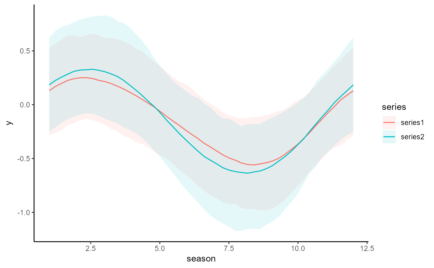
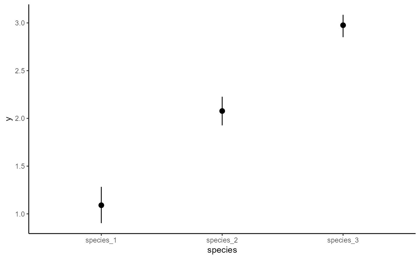
conditional_effects(mod, type = 'expected')
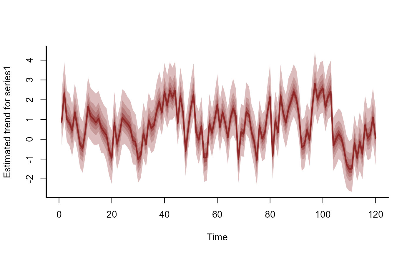
 plot(mod, type = 'trend', series = 1)
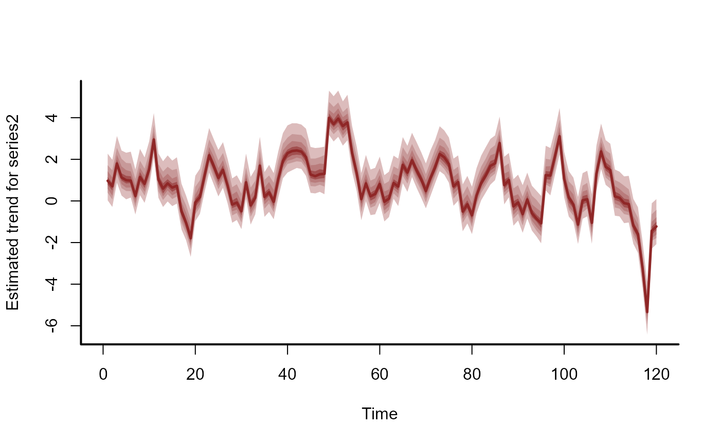
 plot(mod, type = 'trend', series = 2)
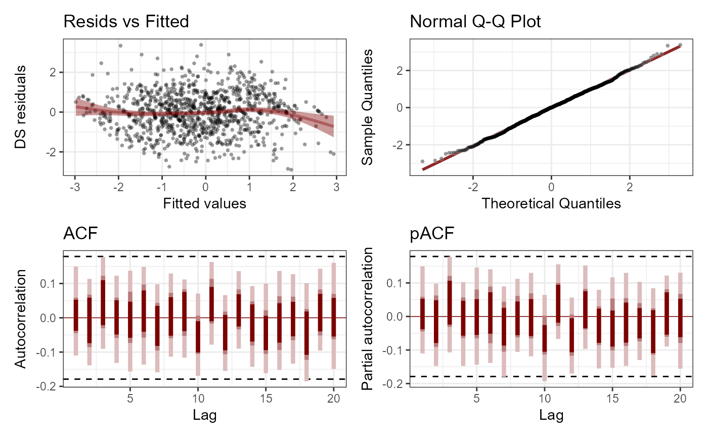
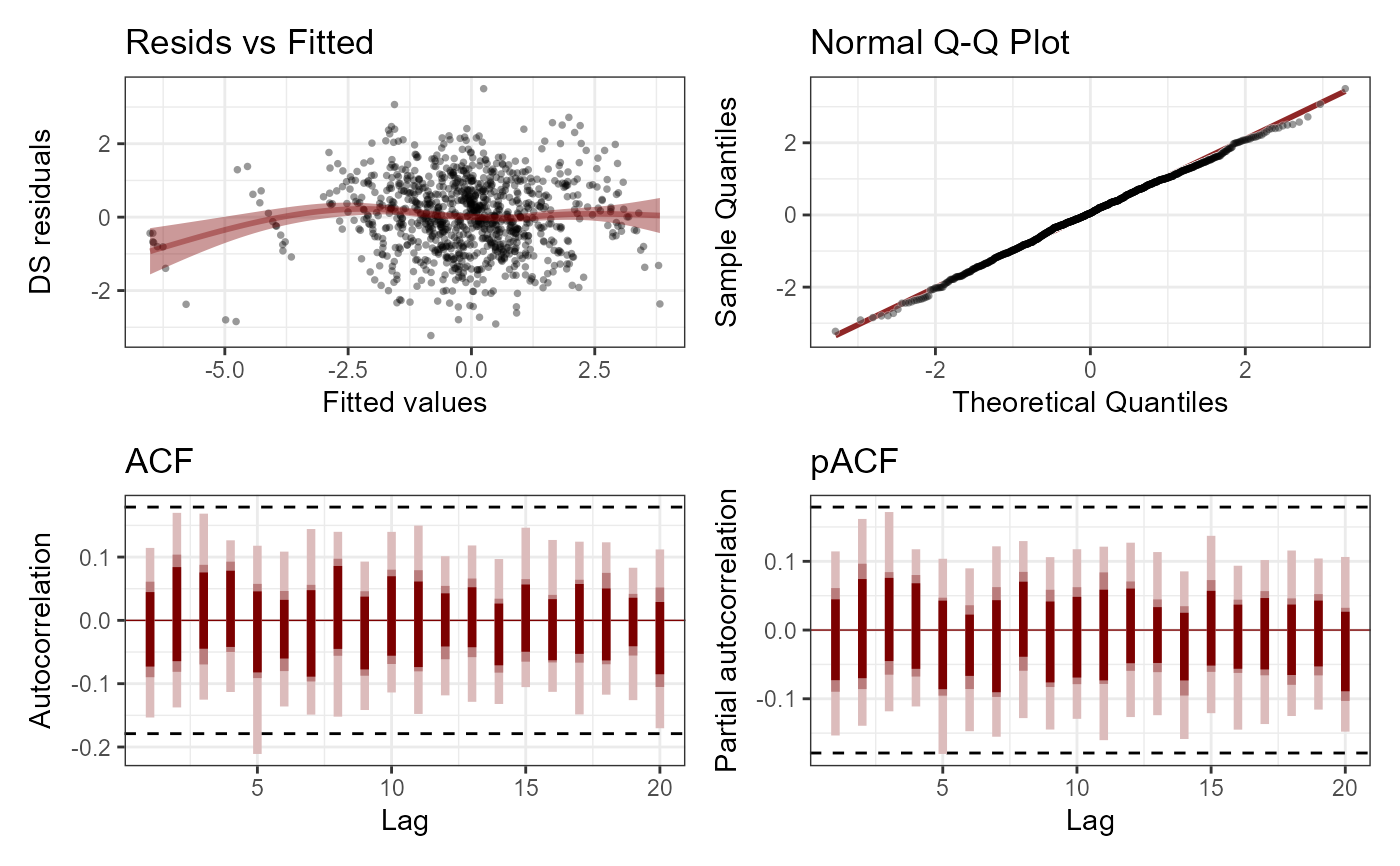
 plot(mod, type = 'residuals', series = 1)
 plot(mod, type = 'residuals', series = 2)
 mcmc_plot(
mod,
variable = 'ar1',
regex = TRUE,
type = 'hist'
)
#> `stat_bin()` using `bins = 30`. Pick better value `binwidth`.
mcmc_plot(
mod,
variable = 'ar1',
regex = TRUE,
type = 'hist'
)
#> `stat_bin()` using `bins = 30`. Pick better value `binwidth`.
 # Now an example illustrating hierarchical dynamics
set.seed(123)
# Simulate three species monitored in three different regions
simdat1 <- sim_mvgam(
trend_model = VAR(cor = TRUE),
prop_trend = 0.95,
n_series = 3,
mu = c(1, 2, 3)
)
simdat2 <- sim_mvgam(
trend_model = VAR(cor = TRUE),
prop_trend = 0.95,
n_series = 3,
mu = c(1, 2, 3)
)
simdat3 <- sim_mvgam(
trend_model = VAR(cor = TRUE),
prop_trend = 0.95,
n_series = 3,
mu = c(1, 2, 3)
)
# Set up the data but DO NOT include 'series'
all_dat <- rbind(
simdat1$data_train %>%
dplyr::mutate(region = 'qld'),
simdat2$data_train %>%
dplyr::mutate(region = 'nsw'),
simdat3$data_train %>%
dplyr::mutate(region = 'vic')
) %>%
dplyr::mutate(
species = gsub('series', 'species', series),
species = as.factor(species),
region = as.factor(region)
) %>%
dplyr::arrange(series, time) %>%
dplyr::select(-series)
# Check priors for a hierarchical AR1 model
get_mvgam_priors(
formula = y ~ species,
trend_model = AR(gr = region, subgr = species),
data = all_dat
)
#> param_name param_length
#> 1 (Intercept) 1
#> 2 speciesspecies_2 1
#> 3 speciesspecies_3 1
#> 4 vector<lower=-1,upper=1>[n_series] ar1; 9
#> 5 vector<lower=0>[n_series] sigma; 9
#> param_info prior
#> 1 (Intercept) (Intercept) ~ student_t(3, 1.9, 2.5);
#> 2 speciesspecies_2 fixed effect speciesspecies_2 ~ student_t(3, 0, 2);
#> 3 speciesspecies_3 fixed effect speciesspecies_3 ~ student_t(3, 0, 2);
#> 4 trend AR1 coefficient ar1 ~ std_normal();
#> 5 trend sd sigma ~ inv_gamma(1.418, 0.452);
#> example_change new_lowerbound new_upperbound
#> 1 (Intercept) ~ normal(0, 1); NA NA
#> 2 speciesspecies_2 ~ normal(0, 1); NA NA
#> 3 speciesspecies_3 ~ normal(0, 1); NA NA
#> 4 ar1 ~ normal(-0.79, 0.86); NA NA
#> 5 sigma ~ exponential(0.37); NA NA
# Fit the model
mod <- mvgam(
formula = y ~ species,
trend_model = AR(gr = region, subgr = species),
data = all_dat,
chains = 2,
silent = 2
)
# Check standard outputs
summary(mod)
#> GAM formula:
#> y ~ species
#> <environment: 0x5582c8b4a668>
#>
#> Family:
#> poisson
#>
#> Link function:
#> log
#>
#> Trend model:
#> AR(gr = region, subgr = species)
#>
#> N series:
#> 9
#>
#> N timepoints:
#> 75
#>
#> Status:
#> Fitted using Stan
#> 2 chains, each with iter = 1000; warmup = 500; thin = 1
#> Total post-warmup draws = 1000
#>
#> GAM coefficient (beta) estimates:
#> 2.5% 50% 97.5% Rhat n_eff
#> (Intercept) 0.92 1.10 1.3 1.03 174
#> speciesspecies_2 0.80 0.98 1.2 1.01 409
#> speciesspecies_3 1.60 1.90 2.1 1.05 70
#>
#> standard deviation:
#> 2.5% 50% 97.5% Rhat n_eff
#> sigma[1] 0.78 0.97 1.20 1.00 574
#> sigma[2] 0.64 0.78 0.95 1.01 569
#> sigma[3] 0.80 0.95 1.20 1.00 571
#> sigma[4] 0.29 0.45 0.68 1.02 110
#> sigma[5] 0.61 0.73 0.89 1.00 671
#> sigma[6] 0.66 0.78 0.94 1.00 616
#> sigma[7] 0.59 0.77 0.99 1.00 357
#> sigma[8] 0.54 0.68 0.88 1.00 448
#> sigma[9] 0.68 0.82 0.99 1.00 720
#>
#> precision parameter:
#> 2.5% 50% 97.5% Rhat n_eff
#> tau[1] 0.65 1.1 1.6 1.00 571
#> tau[2] 1.10 1.6 2.4 1.00 574
#> tau[3] 0.75 1.1 1.5 1.00 544
#> tau[4] 2.20 4.9 12.0 1.02 143
#> tau[5] 1.30 1.9 2.7 1.00 698
#> tau[6] 1.10 1.6 2.3 1.00 641
#> tau[7] 1.00 1.7 2.9 1.00 379
#> tau[8] 1.30 2.2 3.4 1.00 489
#> tau[9] 1.00 1.5 2.2 1.00 770
#>
#> autoregressive coef 1:
#> 2.5% 50% 97.5% Rhat n_eff
#> ar1[1] 0.2500 0.49 0.7100 1.02 129
#> ar1[2] 0.1300 0.34 0.5500 1.01 160
#> ar1[3] 0.0460 0.36 0.6500 1.04 45
#> ar1[4] 0.3000 0.65 0.8700 1.01 158
#> ar1[5] -0.1400 0.09 0.3000 1.00 153
#> ar1[6] -0.4300 -0.21 0.0086 1.00 97
#> ar1[7] -0.0015 0.31 0.6200 1.00 237
#> ar1[8] 0.5400 0.74 0.9100 1.00 129
#> ar1[9] 0.3200 0.54 0.7700 1.01 102
#>
#> Hierarchical correlation weighting parameter (alpha_cor) estimates:
#> 2.5% 50% 97.5% Rhat n_eff
#> alpha_cor 0.014 0.074 0.21 1 332
#>
#> Stan MCMC diagnostics:
#> ✔ No issues with effective samples per iteration
#> ✔ Rhat looks good for all parameters
#> ✔ No issues with divergences
#> ✔ No issues with maximum tree depth
#>
#> Samples were drawn using sampling(hmc). For each parameter, n_eff is a
#> crude measure of effective sample size, and Rhat is the potential scale
#> reduction factor on split MCMC chains (at convergence, Rhat = 1)
#>
#> Use how_to_cite() to get started describing this model
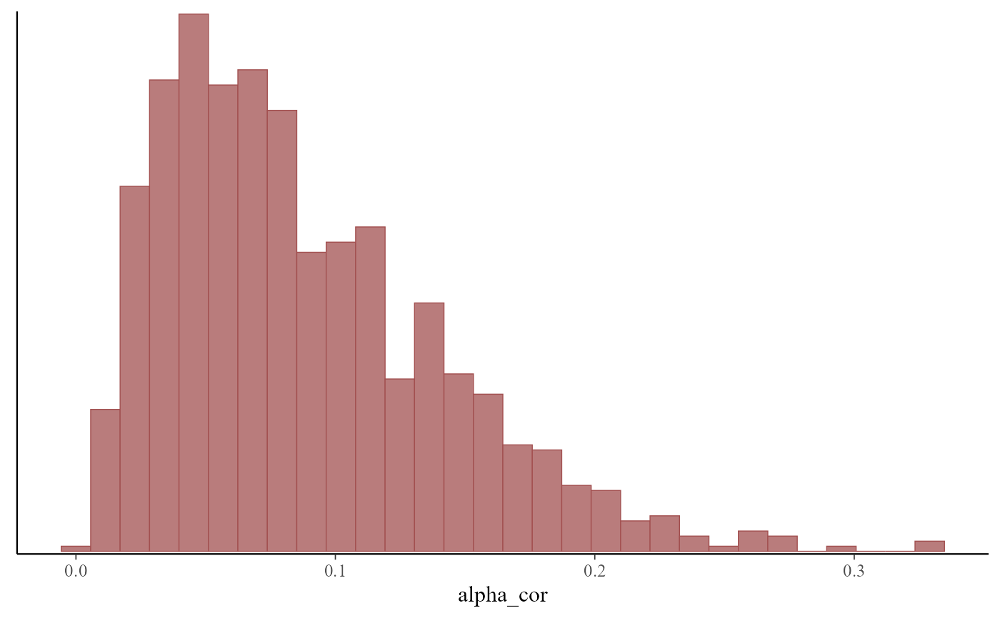
# Inspect posterior estimates for the correlation weighting parameter
mcmc_plot(mod, variable = 'alpha_cor', type = 'hist')
#> `stat_bin()` using `bins = 30`. Pick better value `binwidth`.
# Now an example illustrating hierarchical dynamics
set.seed(123)
# Simulate three species monitored in three different regions
simdat1 <- sim_mvgam(
trend_model = VAR(cor = TRUE),
prop_trend = 0.95,
n_series = 3,
mu = c(1, 2, 3)
)
simdat2 <- sim_mvgam(
trend_model = VAR(cor = TRUE),
prop_trend = 0.95,
n_series = 3,
mu = c(1, 2, 3)
)
simdat3 <- sim_mvgam(
trend_model = VAR(cor = TRUE),
prop_trend = 0.95,
n_series = 3,
mu = c(1, 2, 3)
)
# Set up the data but DO NOT include 'series'
all_dat <- rbind(
simdat1$data_train %>%
dplyr::mutate(region = 'qld'),
simdat2$data_train %>%
dplyr::mutate(region = 'nsw'),
simdat3$data_train %>%
dplyr::mutate(region = 'vic')
) %>%
dplyr::mutate(
species = gsub('series', 'species', series),
species = as.factor(species),
region = as.factor(region)
) %>%
dplyr::arrange(series, time) %>%
dplyr::select(-series)
# Check priors for a hierarchical AR1 model
get_mvgam_priors(
formula = y ~ species,
trend_model = AR(gr = region, subgr = species),
data = all_dat
)
#> param_name param_length
#> 1 (Intercept) 1
#> 2 speciesspecies_2 1
#> 3 speciesspecies_3 1
#> 4 vector<lower=-1,upper=1>[n_series] ar1; 9
#> 5 vector<lower=0>[n_series] sigma; 9
#> param_info prior
#> 1 (Intercept) (Intercept) ~ student_t(3, 1.9, 2.5);
#> 2 speciesspecies_2 fixed effect speciesspecies_2 ~ student_t(3, 0, 2);
#> 3 speciesspecies_3 fixed effect speciesspecies_3 ~ student_t(3, 0, 2);
#> 4 trend AR1 coefficient ar1 ~ std_normal();
#> 5 trend sd sigma ~ inv_gamma(1.418, 0.452);
#> example_change new_lowerbound new_upperbound
#> 1 (Intercept) ~ normal(0, 1); NA NA
#> 2 speciesspecies_2 ~ normal(0, 1); NA NA
#> 3 speciesspecies_3 ~ normal(0, 1); NA NA
#> 4 ar1 ~ normal(-0.79, 0.86); NA NA
#> 5 sigma ~ exponential(0.37); NA NA
# Fit the model
mod <- mvgam(
formula = y ~ species,
trend_model = AR(gr = region, subgr = species),
data = all_dat,
chains = 2,
silent = 2
)
# Check standard outputs
summary(mod)
#> GAM formula:
#> y ~ species
#> <environment: 0x5582c8b4a668>
#>
#> Family:
#> poisson
#>
#> Link function:
#> log
#>
#> Trend model:
#> AR(gr = region, subgr = species)
#>
#> N series:
#> 9
#>
#> N timepoints:
#> 75
#>
#> Status:
#> Fitted using Stan
#> 2 chains, each with iter = 1000; warmup = 500; thin = 1
#> Total post-warmup draws = 1000
#>
#> GAM coefficient (beta) estimates:
#> 2.5% 50% 97.5% Rhat n_eff
#> (Intercept) 0.92 1.10 1.3 1.03 174
#> speciesspecies_2 0.80 0.98 1.2 1.01 409
#> speciesspecies_3 1.60 1.90 2.1 1.05 70
#>
#> standard deviation:
#> 2.5% 50% 97.5% Rhat n_eff
#> sigma[1] 0.78 0.97 1.20 1.00 574
#> sigma[2] 0.64 0.78 0.95 1.01 569
#> sigma[3] 0.80 0.95 1.20 1.00 571
#> sigma[4] 0.29 0.45 0.68 1.02 110
#> sigma[5] 0.61 0.73 0.89 1.00 671
#> sigma[6] 0.66 0.78 0.94 1.00 616
#> sigma[7] 0.59 0.77 0.99 1.00 357
#> sigma[8] 0.54 0.68 0.88 1.00 448
#> sigma[9] 0.68 0.82 0.99 1.00 720
#>
#> precision parameter:
#> 2.5% 50% 97.5% Rhat n_eff
#> tau[1] 0.65 1.1 1.6 1.00 571
#> tau[2] 1.10 1.6 2.4 1.00 574
#> tau[3] 0.75 1.1 1.5 1.00 544
#> tau[4] 2.20 4.9 12.0 1.02 143
#> tau[5] 1.30 1.9 2.7 1.00 698
#> tau[6] 1.10 1.6 2.3 1.00 641
#> tau[7] 1.00 1.7 2.9 1.00 379
#> tau[8] 1.30 2.2 3.4 1.00 489
#> tau[9] 1.00 1.5 2.2 1.00 770
#>
#> autoregressive coef 1:
#> 2.5% 50% 97.5% Rhat n_eff
#> ar1[1] 0.2500 0.49 0.7100 1.02 129
#> ar1[2] 0.1300 0.34 0.5500 1.01 160
#> ar1[3] 0.0460 0.36 0.6500 1.04 45
#> ar1[4] 0.3000 0.65 0.8700 1.01 158
#> ar1[5] -0.1400 0.09 0.3000 1.00 153
#> ar1[6] -0.4300 -0.21 0.0086 1.00 97
#> ar1[7] -0.0015 0.31 0.6200 1.00 237
#> ar1[8] 0.5400 0.74 0.9100 1.00 129
#> ar1[9] 0.3200 0.54 0.7700 1.01 102
#>
#> Hierarchical correlation weighting parameter (alpha_cor) estimates:
#> 2.5% 50% 97.5% Rhat n_eff
#> alpha_cor 0.014 0.074 0.21 1 332
#>
#> Stan MCMC diagnostics:
#> ✔ No issues with effective samples per iteration
#> ✔ Rhat looks good for all parameters
#> ✔ No issues with divergences
#> ✔ No issues with maximum tree depth
#>
#> Samples were drawn using sampling(hmc). For each parameter, n_eff is a
#> crude measure of effective sample size, and Rhat is the potential scale
#> reduction factor on split MCMC chains (at convergence, Rhat = 1)
#>
#> Use how_to_cite() to get started describing this model
# Inspect posterior estimates for the correlation weighting parameter
mcmc_plot(mod, variable = 'alpha_cor', type = 'hist')
#> `stat_bin()` using `bins = 30`. Pick better value `binwidth`.
 # }
# }