Calculate latent VAR forecast error variance decompositions

Compute forecast error variance decompositions from mvgam models with Vector Autoregressive dynamics

Usage

fevd(object, ...)

# S3 method for mvgam
fevd(object, h = 10, ...)

Arguments

object: list object of class mvgam resulting from a call to mvgam() that used a Vector Autoregressive latent process model (either as VAR(cor = FALSE) or VAR(cor = TRUE))
...: ignored
h: Positive integer specifying the forecast horizon over which to calculate the IRF

Value

An object of class mvgam_fevd containing the posterior forecast error variance decompositions. This object can be used with the supplied S3 functions plot

Details

A forecast error variance decomposition is useful for quantifying the amount of information each series that in a Vector Autoregression contributes to the forecast distributions of the other series in the autoregression. This function calculates the forecast error variance decomposition using the orthogonalised impulse response coefficient matrices $\Psi_h$ , which can be used to quantify the contribution of series $j$ to the h-step forecast error variance of series $k$ : $\sigma_k^2(h) = \sum_{j=1}^K(\psi_{kj, 0}^2 + \ldots + \psi_{kj, h-1}^2) \quad$ If the orthogonalised impulse reponses $(\psi_{kj, 0}^2 + \ldots + \psi_{kj, h-1}^2)$ are divided by the variance of the forecast error $\sigma_k^2(h)$ , this yields an interpretable percentage representing how much of the forecast error variance for $k$ can be explained by an exogenous shock to $j$ .

References

Lütkepohl, H (2006). New Introduction to Multiple Time Series Analysis. Springer, New York.

Author

Nicholas J Clark

Examples

# \donttest{
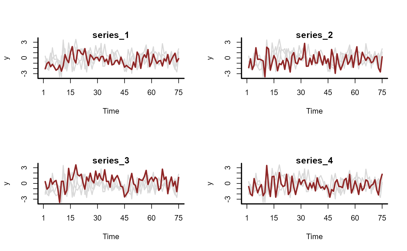
# Simulate some time series that follow a latent VAR(1) process
simdat <- sim_mvgam(
  family = gaussian(),
  n_series = 4,
  trend_model = VAR(cor = TRUE),
  prop_trend = 1
)
plot_mvgam_series(data = simdat$data_train, series = "all")


# Fit a model that uses a latent VAR(1)
mod <- mvgam(y ~ -1,
  trend_formula = ~1,
  trend_model = VAR(cor = TRUE),
  family = gaussian(),
  data = simdat$data_train,
  chains = 2,
  silent = 2
)

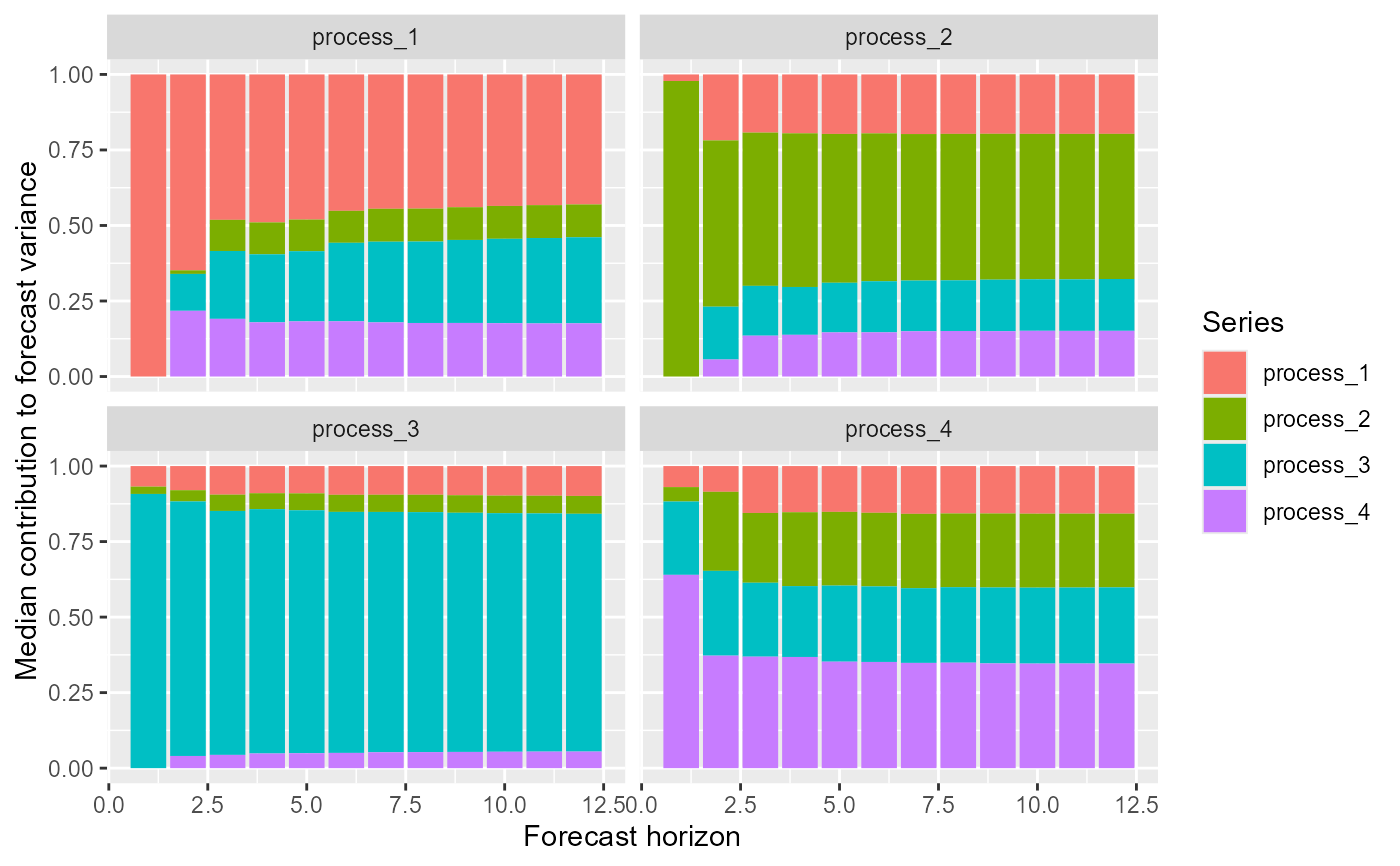# Calulate forecast error variance decompositions for each series
fevds <- fevd(mod, h = 12)

# Plot median contributions to forecast error variance
plot(fevds)


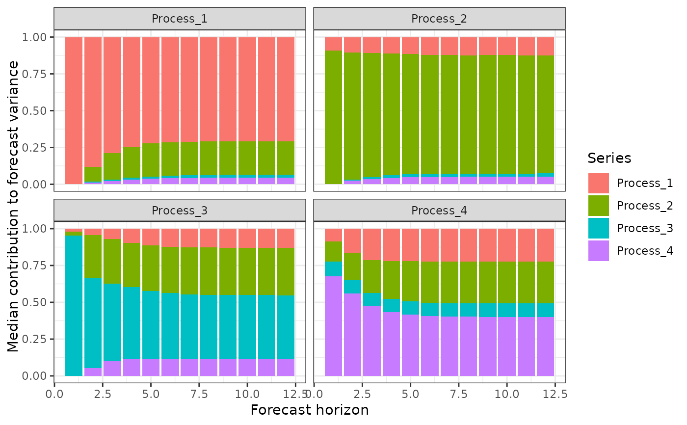# View a summary of the error variance decompositions
summary(fevds)
#> # A tibble: 192 × 5
#>    shock                  horizon fevdQ50 fevdQ2.5 fevdQ97.5
#>    <chr>                    <int>   <dbl>    <dbl>     <dbl>
#>  1 Process_1 -> Process_1       1   1        1         1    
#>  2 Process_1 -> Process_1       2   0.861    0.500     0.986
#>  3 Process_1 -> Process_1       3   0.763    0.376     0.969
#>  4 Process_1 -> Process_1       4   0.708    0.313     0.957
#>  5 Process_1 -> Process_1       5   0.686    0.279     0.950
#>  6 Process_1 -> Process_1       6   0.677    0.271     0.946
#>  7 Process_1 -> Process_1       7   0.672    0.271     0.944
#>  8 Process_1 -> Process_1       8   0.669    0.273     0.942
#>  9 Process_1 -> Process_1       9   0.668    0.269     0.942
#> 10 Process_1 -> Process_1      10   0.668    0.268     0.941
#> # ℹ 182 more rows
# }

References

Lütkepohl, H. (2007). New Introduction to Multiple Time Series Analysis. 2nd ed. Springer-Verlag Berlin Heidelberg.