Supported mvgam families

Usage

tweedie(link = "log")

student_t(link = "identity")

nmix(link = "log")

Arguments

link: a specification for the family link function. At present these cannot be changed

Details

mvgam currently supports the following standard observation families:

gaussian with identity link, for real-valued data
poisson with log-link, for count data
Gamma with log-link, for non-negative real-valued data
binomial with logit-link, for count data when the number of trials is known (and must be supplied)

In addition, the following extended families from the mgcv and brms packages are supported:

betar with logit-link, for proportional data on (0,1)
nb with log-link, for count data
lognormal with identity-link, for non-negative real-valued data
bernoulli with logit-link, for binary data

Finally, mvgam supports the three extended families described here:

tweedie with log-link, for count data (power parameter p fixed at 1.5)
student_t() (or student) with identity-link, for real-valued data
nmix for count data with imperfect detection modeled via a State-Space N-Mixture model. The latent states are Poisson (with log link), capturing the 'true' latent abundance, while the observation process is Binomial to account for imperfect detection. The observation formula in these models is used to set up a linear predictor for the detection probability (with logit link). See the example below for a more detailed worked explanation of the nmix() family

Only poisson(), nb(), and tweedie() are available if using JAGS. All families, apart from tweedie(), are supported if using Stan.

Note that currently it is not possible to change the default link functions in mvgam, so any call to change these will be silently ignored

Author

Nicholas J Clark

Examples

if (FALSE) {
# Example showing how to set up N-mixture models
set.seed(999)
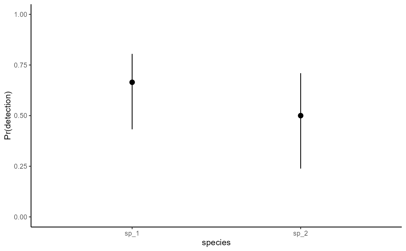
# Simulate observations for species 1, which shows a declining trend and 0.7 detection probability
data.frame(site = 1,
          # five replicates per year; six years
          replicate = rep(1:5, 6),
          time = sort(rep(1:6, 5)),
          species = 'sp_1',
          # true abundance declines nonlinearly
          truth = c(rep(28, 5),
                    rep(26, 5),
                    rep(23, 5),
                    rep(16, 5),
                    rep(14, 5),
                    rep(14, 5)),
          # observations are taken with detection prob = 0.7
          obs = c(rbinom(5, 28, 0.7),
                  rbinom(5, 26, 0.7),
                  rbinom(5, 23, 0.7),
                  rbinom(5, 15, 0.7),
                  rbinom(5, 14, 0.7),
                  rbinom(5, 14, 0.7))) %>%
 # add 'series' information, which is an identifier of site, replicate and species
 dplyr::mutate(series = paste0('site_', site,
                               '_', species,
                               '_rep_', replicate),
               time = as.numeric(time),
               # add a 'cap' variable that defines the maximum latent N to
               # marginalize over when estimating latent abundance; in other words
               # how large do we realistically think the true abundance could be?
               cap = 80) %>%
 dplyr::select(- replicate) -> testdat

# Now add another species that has a different temporal trend and a smaller
# detection probability (0.45 for this species)
testdat = testdat %>%
 dplyr::bind_rows(data.frame(site = 1,
                             replicate = rep(1:5, 6),
                             time = sort(rep(1:6, 5)),
                             species = 'sp_2',
                             truth = c(rep(4, 5),
                                       rep(7, 5),
                                       rep(15, 5),
                                       rep(16, 5),
                                       rep(19, 5),
                                       rep(18, 5)),
                             obs = c(rbinom(5, 4, 0.45),
                                     rbinom(5, 7, 0.45),
                                     rbinom(5, 15, 0.45),
                                     rbinom(5, 16, 0.45),
                                     rbinom(5, 19, 0.45),
                                     rbinom(5, 18, 0.45))) %>%
                    dplyr::mutate(series = paste0('site_', site,
                                                  '_', species,
                                                  '_rep_', replicate),
                                  time = as.numeric(time),
                                  cap = 50) %>%
                    dplyr::select(-replicate))

# series identifiers
testdat$species <- factor(testdat$species,
                          levels = unique(testdat$species))
testdat$series <- factor(testdat$series,
                         levels = unique(testdat$series))

# The trend_map to state how replicates are structured
testdat %>%
# each unique combination of site*species is a separate process
dplyr::mutate(trend = as.numeric(factor(paste0(site, species)))) %>%
 dplyr::select(trend, series) %>%
 dplyr::distinct() -> trend_map
trend_map

# Fit a model
mod <- mvgam(
            # the observation formula sets up linear predictors for
            # detection probability on the logit scale
            formula = obs ~ species - 1,

            # the trend_formula sets up the linear predictors for
            # the latent abundance processes on the log scale
            trend_formula = ~ s(time, by = trend, k = 4) + species,

            # the trend_map takes care of the mapping
            trend_map = trend_map,

            # nmix() family and data
            family = nmix(),
            data = testdat,

            # priors can be set in the usual way
            priors = c(prior(std_normal(), class = b),
                       prior(normal(1, 1.5), class = Intercept_trend)),
            burnin = 300,
            samples = 300,
            chains = 2)

# The usual diagnostics
summary(mod)

# Plotting conditional effects
library(ggplot2)
plot_predictions(mod, condition = 'species',
                 type = 'detection') +
     ylab('Pr(detection)') +
     ylim(c(0, 1)) +
     theme_classic() +
     theme(legend.position = 'none')

# Example showcasing how cbind() is needed for Binomial observations
# Simulate two time series of Binomial trials
trials <- sample(c(20:25), 50, replace = TRUE)
x <- rnorm(50)
detprob1 <- plogis(-0.5 + 0.9*x)
detprob2 <- plogis(-0.1 -0.7*x)
dat <- rbind(data.frame(y = rbinom(n = 50, size = trials, prob = detprob1),
                        time = 1:50,
                        series = 'series1',
                        x = x,
                        ntrials = trials),
             data.frame(y = rbinom(n = 50, size = trials, prob = detprob2),
                        time = 1:50,
                        series = 'series2',
                        x = x,
                        ntrials = trials))
dat <- dplyr::mutate(dat, series = as.factor(series))
dat <- dplyr::arrange(dat, time, series)

# Fit a model using the binomial() family; must specify observations
# and number of trials in the cbind() wrapper
mod <- mvgam(cbind(y, ntrials) ~ series + s(x, by = series),
             family = binomial(),
             data = dat)
summary(mod)
}