Time-varying effects in mvgam

The purpose of this vignette is to show how the mvgam package can be used to estimate and forecast regression coefficients that vary through time.

Time-varying effects

Dynamic fixed-effect coefficients (often referred to as dynamic linear models) can be readily incorporated into GAMs / DGAMs. In mvgam, the dynamic() formula wrapper offers a convenient interface to set these up. The plan is to incorporate a range of dynamic options (such as random walk, AR1 etc…) but for the moment only low-rank Gaussian Process (GP) smooths are allowed (making use either of the gp basis in mgcv of of Hilbert space approximate GPs). These are advantageous over splines or random walk effects for several reasons. First, GPs will force the time-varying effect to be smooth. This often makes sense in reality, where we would not expect a regression coefficient to change rapidly from one time point to the next. Second, GPs provide information on the ‘global’ dynamics of a time-varying effect through their length-scale parameters. This means we can use them to provide accurate forecasts of how an effect is expected to change in the future, something that we couldn’t do well if we used splines to estimate the effect. An example below illustrates.

Simulating time-varying effects

Simulate a time-varying coefficient using a squared exponential Gaussian Process function with length scale \(\rho\)=10. We will do this using an internal function from mvgam (the sim_gp function):

set.seed(1111)
N <- 200
beta_temp <- mvgam:::sim_gp(rnorm(1),
                            alpha_gp = 0.75,
                            rho_gp = 10,
                            h = N) + 0.5

A plot of the time-varying coefficient shows that it changes smoothly through time:

plot(beta_temp, type = 'l', lwd = 3, 
     bty = 'l', xlab = 'Time', ylab = 'Coefficient',
     col = 'darkred')
box(bty = 'l', lwd = 2)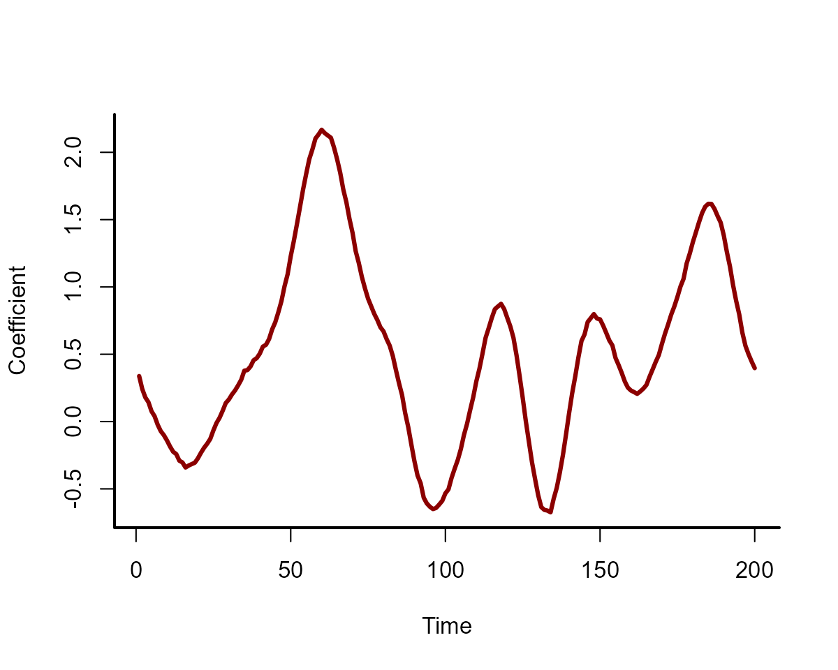

Simulating time-varying effects in mvgam and R

Next we need to simulate the values of the covariate, which we will call temp (to represent \(temperature\)). In this case we just use a standard normal distribution to simulate this covariate:

temp <- rnorm(N, sd = 1)

Finally, simulate the outcome variable, which is a Gaussian observation process (with observation error) over the time-varying effect of \(temperature\)

out <- rnorm(N, mean = 4 + beta_temp * temp,
             sd = 0.25)
time <- seq_along(temp)
plot(out,  type = 'l', lwd = 3, 
     bty = 'l', xlab = 'Time', ylab = 'Outcome',
     col = 'darkred')
box(bty = 'l', lwd = 2)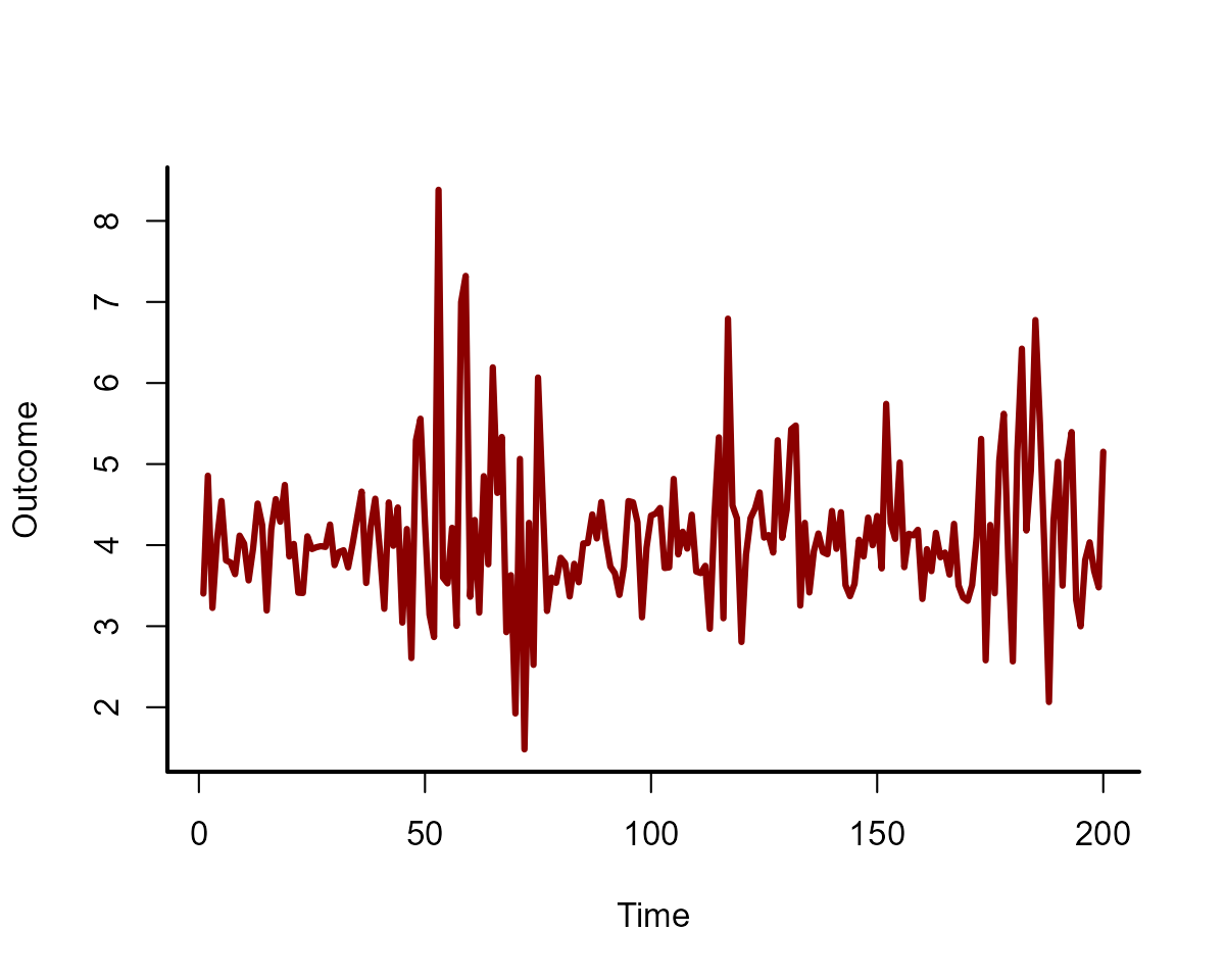

Simulating time-varying effects in mvgam and R

Gather the data into a data.frame for fitting models, and split the data into training and testing folds.

data <- data.frame(out, temp, time)
data_train <- data[1:190,]
data_test <- data[191:200,]

Plot the series

plot_mvgam_series(data = data_train, newdata = data_test, y = 'out')

The `dynamic()` function

Time-varying coefficients can be fairly easily set up using the s() or gp() wrapper functions in mvgam formulae by fitting a nonlinear effect of time and using the covariate of interest as the numeric by variable (see ?mgcv::s or ?brms::gp for more details). The dynamic() formula wrapper offers a way to automate this process, and will eventually allow for a broader variety of time-varying effects (such as random walk or AR processes). Depending on the arguments that are specified to dynamic, it will either set up a low-rank GP smooth function using s() with bs = 'gp' and a fixed value of the length scale parameter \(\rho\), or it will set up a Hilbert space approximate GP using the gp() function with c=5/4 so that \(\rho\) is estimated (see ?dynamic for more details). In this first example we will use the s() option, and will mis-specify the \(\rho\) parameter here as, in practice, it is never known. This call to dynamic() will set up the following smooth: s(time, by = temp, bs = "gp", m = c(-2, 8, 2), k = 40)

mod <- mvgam(out ~ dynamic(temp, rho = 8, stationary = TRUE, k = 40),
             family = gaussian(),
             data = data_train)

Inspect the model summary, which shows how the dynamic() wrapper was used to construct a low-rank Gaussian Process smooth function:

summary(mod, include_betas = FALSE)

## GAM formula:
## out ~ s(time, by = temp, bs = "gp", m = c(-2, 8, 2), k = 40)
## 
## Family:
## gaussian
## 
## Link function:
## identity
## 
## Trend model:
## None
## 
## N series:
## 1 
## 
## N timepoints:
## 190 
## 
## Status:
## Fitted using Stan 
## 4 chains, each with iter = 1000; warmup = 500; thin = 1 
## Total post-warmup draws = 2000
## 
## 
## Observation error parameter estimates:
##              2.5%  50% 97.5% Rhat n_eff
## sigma_obs[1] 0.23 0.25  0.28    1  2222
## 
## GAM coefficient (beta) estimates:
##             2.5% 50% 97.5% Rhat n_eff
## (Intercept)    4   4   4.1    1  2893
## 
## Approximate significance of GAM observation smooths:
##              edf Ref.df    F p-value    
## s(time):temp  14     40 72.4  <2e-16 ***
## ---
## Signif. codes:  0 '***' 0.001 '**' 0.01 '*' 0.05 '.' 0.1 ' ' 1
## 
## Stan MCMC diagnostics:
## n_eff / iter looks reasonable for all parameters
## Rhat looks reasonable for all parameters
## 0 of 2000 iterations ended with a divergence (0%)
## 0 of 2000 iterations saturated the maximum tree depth of 12 (0%)
## E-FMI indicated no pathological behavior
## 
## Samples were drawn using NUTS(diag_e) at Mon Mar 25 2:43:44 PM 2024.
## For each parameter, n_eff is a crude measure of effective sample size,
## and Rhat is the potential scale reduction factor on split MCMC chains
## (at convergence, Rhat = 1)

Because this model used a spline with a gp basis, it’s smooths can be visualised just like any other gam. Plot the estimated time-varying coefficient for the in-sample training period

plot(mod, type = 'smooths')

We can also plot the estimates for the in-sample and out-of-sample periods to see how the Gaussian Process function produces sensible smooth forecasts. Here we supply the full dataset to the newdata argument in plot_mvgam_smooth to inspect posterior forecasts of the time-varying smooth function. Overlay the true simulated function to see that the model has adequately estimated it’s dynamics in both the training and testing data partitions

plot_mvgam_smooth(mod, smooth = 1, newdata = data)
abline(v = 190, lty = 'dashed', lwd = 2)
lines(beta_temp, lwd = 2.5, col = 'white')
lines(beta_temp, lwd = 2)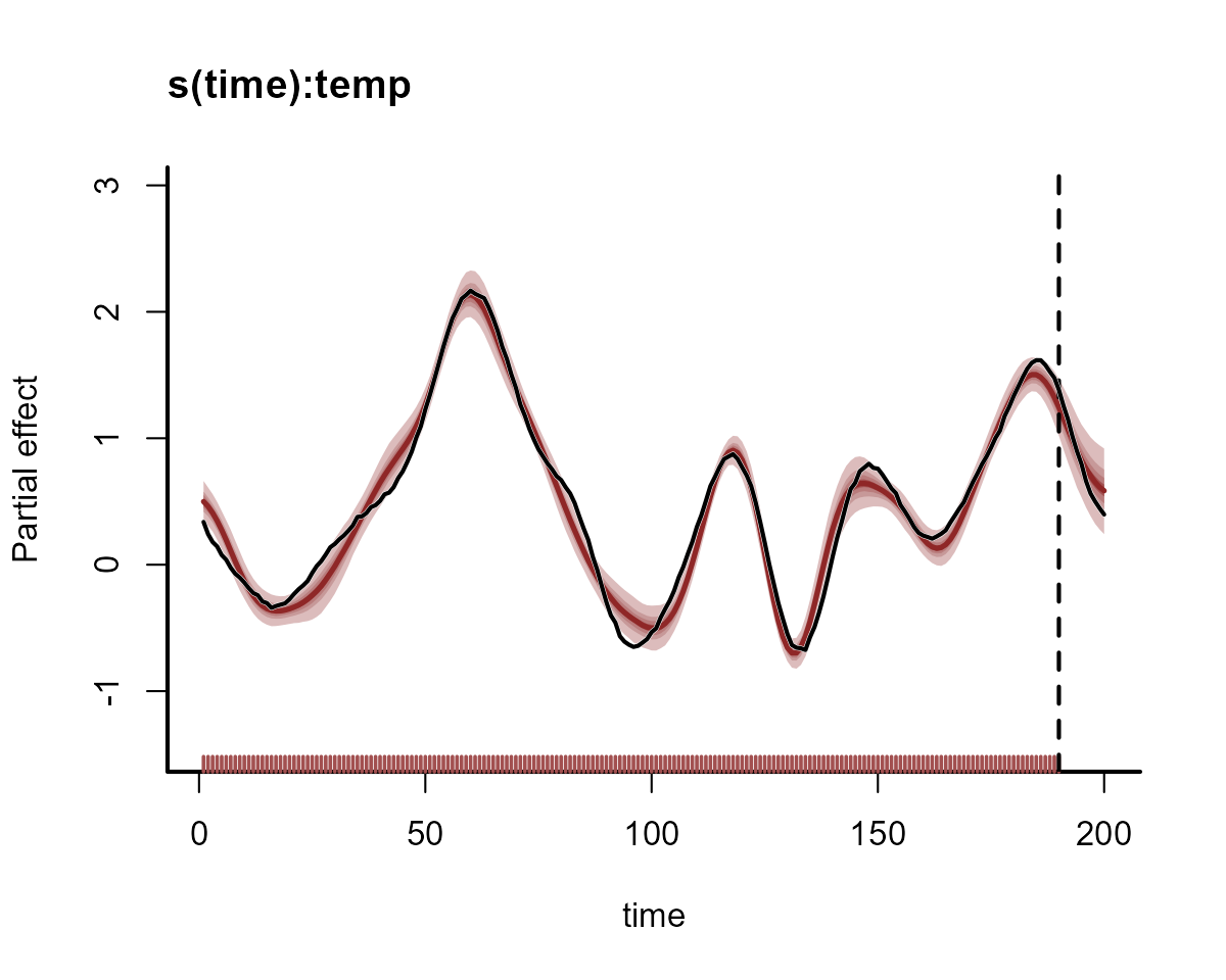

We can also use plot_predictions from the marginaleffects package to visualise the time-varying coefficient for what the effect would be estimated to be at different values of \(temperature\):

range_round = function(x){
  round(range(x, na.rm = TRUE), 2)
}
plot_predictions(mod, 
                 newdata = datagrid(time = unique,
                                    temp = range_round),
                 by = c('time', 'temp', 'temp'),
                 type = 'link')

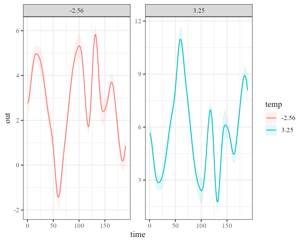
This results in sensible forecasts of the observations as well

plot(mod, type = 'forecast', newdata = data_test)

## Out of sample CRPS:
## [1] 1.280347

The syntax is very similar if we wish to estimate the parameters of the underlying Gaussian Process, this time using a Hilbert space approximation. We simply omit the rho argument in dynamic to make this happen. This will set up a call similar to gp(time, by = 'temp', c = 5/4, k = 40).

mod <- mvgam(out ~ dynamic(temp, k = 40),
             family = gaussian(),
             data = data_train)

This model summary now contains estimates for the marginal deviation and length scale parameters of the underlying Gaussian Process function:

summary(mod, include_betas = FALSE)

## GAM formula:
## out ~ gp(time, by = temp, c = 5/4, k = 40, scale = TRUE)
## 
## Family:
## gaussian
## 
## Link function:
## identity
## 
## Trend model:
## None
## 
## N series:
## 1 
## 
## N timepoints:
## 190 
## 
## Status:
## Fitted using Stan 
## 4 chains, each with iter = 1000; warmup = 500; thin = 1 
## Total post-warmup draws = 2000
## 
## 
## Observation error parameter estimates:
##              2.5%  50% 97.5% Rhat n_eff
## sigma_obs[1] 0.24 0.26  0.29    1  2151
## 
## GAM coefficient (beta) estimates:
##             2.5% 50% 97.5% Rhat n_eff
## (Intercept)    4   4   4.1    1  2989
## 
## GAM gp term marginal deviation (alpha) and length scale (rho) estimates:
##                      2.5%   50% 97.5% Rhat n_eff
## alpha_gp(time):temp 0.640 0.890 1.400 1.01   745
## rho_gp(time):temp   0.028 0.053 0.069 1.00   888
## 
## Stan MCMC diagnostics:
## n_eff / iter looks reasonable for all parameters
## Rhat looks reasonable for all parameters
## 1 of 2000 iterations ended with a divergence (0.05%)
##  *Try running with larger adapt_delta to remove the divergences
## 0 of 2000 iterations saturated the maximum tree depth of 12 (0%)
## E-FMI indicated no pathological behavior
## 
## Samples were drawn using NUTS(diag_e) at Mon Mar 25 2:44:41 PM 2024.
## For each parameter, n_eff is a crude measure of effective sample size,
## and Rhat is the potential scale reduction factor on split MCMC chains
## (at convergence, Rhat = 1)

Effects for gp() terms can also be plotted as smooths:

plot_mvgam_smooth(mod, smooth = 1, newdata = data)
abline(v = 190, lty = 'dashed', lwd = 2)
lines(beta_temp, lwd = 2.5, col = 'white')
lines(beta_temp, lwd = 2)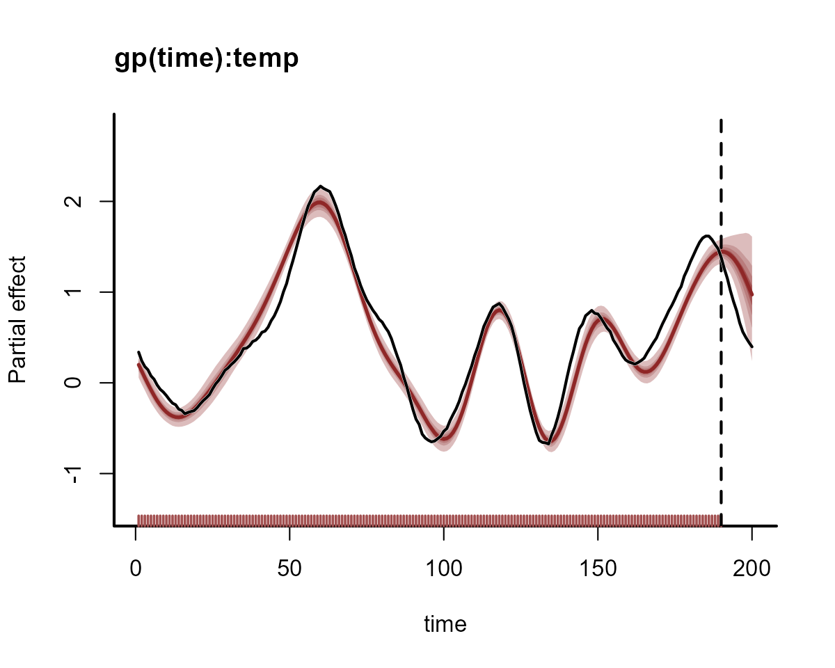

Both the above plot and the below plot_predictions() call show that the effect in this case is similar to what we estimated in the approximate GP smooth model above:

plot_predictions(mod, 
                 newdata = datagrid(time = unique,
                                    temp = range_round),
                 by = c('time', 'temp', 'temp'),
                 type = 'link')

Forecasts are also similar:

plot(mod, type = 'forecast', newdata = data_test)

## Out of sample CRPS:
## [1] 1.667521

Salmon survival example

Here we will use openly available data on marine survival of Chinook salmon to illustrate how time-varying effects can be used to improve ecological time series models. Scheuerell and Williams (2005) used a dynamic linear model to examine the relationship between marine survival of Chinook salmon and an index of ocean upwelling strength along the west coast of the USA. The authors hypothesized that stronger upwelling in April should create better growing conditions for phytoplankton, which would then translate into more zooplankton and provide better foraging opportunities for juvenile salmon entering the ocean. The data on survival is measured as a proportional variable over 42 years (1964–2005) and is available in the MARSS package:

load(url('https://github.com/atsa-es/MARSS/raw/master/data/SalmonSurvCUI.rda'))
dplyr::glimpse(SalmonSurvCUI)

## Rows: 42
## Columns: 3
## $ year    <int> 1964, 1965, 1966, 1967, 1968, 1969, 1970, 1971, 1972, 1973, 19…
## $ logit.s <dbl> -3.46, -3.32, -3.58, -3.03, -3.61, -3.35, -3.93, -4.19, -4.82,…
## $ CUI.apr <int> 57, 5, 43, 11, 47, -21, 25, -2, -1, 43, 2, 35, 0, 1, -1, 6, -7…

First we need to prepare the data for modelling. The variable CUI.apr will be standardized to make it easier for the sampler to estimate underlying GP parameters for the time-varying effect. We also need to convert the survival back to a proportion, as in its current form it has been logit-transformed (this is because most time series packages cannot handle proportional data). As usual, we also need to create a time indicator and a series indicator for working in mvgam:

SalmonSurvCUI %>%
  # create a time variable
  dplyr::mutate(time = dplyr::row_number()) %>%

  # create a series variable
  dplyr::mutate(series = as.factor('salmon')) %>%

  # z-score the covariate CUI.apr
  dplyr::mutate(CUI.apr = as.vector(scale(CUI.apr))) %>%

  # convert logit-transformed survival back to proportional
  dplyr::mutate(survival = plogis(logit.s)) -> model_data

Inspect the data

dplyr::glimpse(model_data)

## Rows: 42
## Columns: 6
## $ year     <int> 1964, 1965, 1966, 1967, 1968, 1969, 1970, 1971, 1972, 1973, 1…
## $ logit.s  <dbl> -3.46, -3.32, -3.58, -3.03, -3.61, -3.35, -3.93, -4.19, -4.82…
## $ CUI.apr  <dbl> 2.37949804, 0.03330223, 1.74782994, 0.30401713, 1.92830654, -…
## $ time     <int> 1, 2, 3, 4, 5, 6, 7, 8, 9, 10, 11, 12, 13, 14, 15, 16, 17, 18…
## $ series   <fct> salmon, salmon, salmon, salmon, salmon, salmon, salmon, salmo…
## $ survival <dbl> 0.030472033, 0.034891409, 0.027119717, 0.046088827, 0.0263393…

Plot features of the outcome variable, which shows that it is a proportional variable with particular restrictions that we want to model:

plot_mvgam_series(data = model_data, y = 'survival')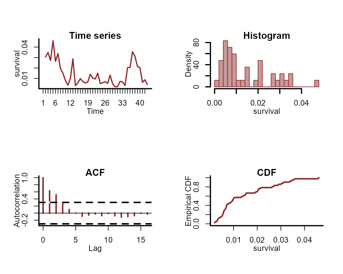

A State-Space Beta regression

mvgam can easily handle data that are bounded at 0 and 1 with a Beta observation model (using the mgcv function betar(), see ?mgcv::betar for details). First we will fit a simple State-Space model that uses a Random Walk dynamic process model with no predictors and a Beta observation model:

mod0 <- mvgam(formula = survival ~ 1,
             trend_model = 'RW',
             family = betar(),
             data = model_data)

The summary of this model shows good behaviour of the Hamiltonian Monte Carlo sampler and provides useful summaries on the Beta observation model parameters:

summary(mod0)

## GAM formula:
## survival ~ 1
## 
## Family:
## beta
## 
## Link function:
## logit
## 
## Trend model:
## RW
## 
## N series:
## 1 
## 
## N timepoints:
## 42 
## 
## Status:
## Fitted using Stan 
## 4 chains, each with iter = 1000; warmup = 500; thin = 1 
## Total post-warmup draws = 2000
## 
## 
## Observation precision parameter estimates:
##        2.5% 50% 97.5% Rhat n_eff
## phi[1]  160 310   580 1.01   612
## 
## GAM coefficient (beta) estimates:
##             2.5%  50% 97.5% Rhat n_eff
## (Intercept) -4.2 -3.4  -2.4 1.02   125
## 
## Latent trend variance estimates:
##          2.5%  50% 97.5% Rhat n_eff
## sigma[1] 0.18 0.33  0.55 1.02   276
## 
## Stan MCMC diagnostics:
## n_eff / iter looks reasonable for all parameters
## Rhat looks reasonable for all parameters
## 0 of 2000 iterations ended with a divergence (0%)
## 0 of 2000 iterations saturated the maximum tree depth of 12 (0%)
## E-FMI indicated no pathological behavior
## 
## Samples were drawn using NUTS(diag_e) at Mon Mar 25 2:45:37 PM 2024.
## For each parameter, n_eff is a crude measure of effective sample size,
## and Rhat is the potential scale reduction factor on split MCMC chains
## (at convergence, Rhat = 1)

A plot of the underlying dynamic component shows how it has easily handled the temporal evolution of the time series:

plot(mod0, type = 'trend')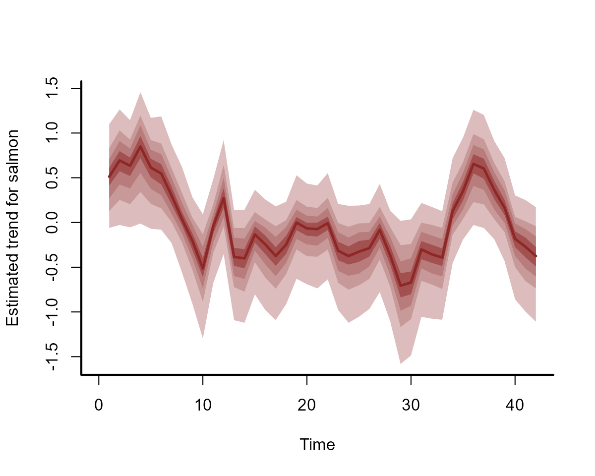

Posterior hindcasts are also good and will automatically respect the observational data bounding at 0 and 1:

plot(mod0, type = 'forecast')

Including time-varying upwelling effects

Now we can increase the complexity of our model by constructing and fitting a State-Space model with a time-varying effect of the coastal upwelling index in addition to the autoregressive dynamics. We again use a Beta observation model to capture the restrictions of our proportional observations, but this time will include a dynamic() effect of CUI.apr in the latent process model. We do not specify the \(\rho\) parameter, instead opting to estimate it using a Hilbert space approximate GP:

mod1 <- mvgam(formula = survival ~ 1,
              trend_formula = ~ dynamic(CUI.apr, k = 25, scale = FALSE),
              trend_model = 'RW',
              family = betar(),
              data = model_data)

The summary for this model now includes estimates for the time-varying GP parameters:

summary(mod1, include_betas = FALSE)

## GAM observation formula:
## survival ~ 1
## 
## GAM process formula:
## ~dynamic(CUI.apr, k = 25, scale = FALSE)
## 
## Family:
## beta
## 
## Link function:
## logit
## 
## Trend model:
## RW
## 
## N process models:
## 1 
## 
## N series:
## 1 
## 
## N timepoints:
## 42 
## 
## Status:
## Fitted using Stan 
## 4 chains, each with iter = 1000; warmup = 500; thin = 1 
## Total post-warmup draws = 2000
## 
## 
## Observation precision parameter estimates:
##        2.5% 50% 97.5% Rhat n_eff
## phi[1]  190 360   670    1   858
## 
## GAM observation model coefficient (beta) estimates:
##             2.5%  50% 97.5% Rhat n_eff
## (Intercept) -4.1 -3.2  -2.2 1.07    64
## 
## Process error parameter estimates:
##          2.5%  50% 97.5% Rhat n_eff
## sigma[1] 0.18 0.31  0.51 1.02   274
## 
## GAM process model gp term marginal deviation (alpha) and length scale (rho) estimates:
##                                2.5%  50% 97.5% Rhat n_eff
## alpha_gp_time_byCUI_apr_trend 0.028 0.32   1.5 1.02   205
## rho_gp_time_byCUI_apr_trend   1.400 6.50  40.0 1.02   236
## 
## Stan MCMC diagnostics:
## n_eff / iter looks reasonable for all parameters
## Rhats above 1.05 found for 30 parameters
##  *Diagnose further to investigate why the chains have not mixed
## 89 of 2000 iterations ended with a divergence (4.45%)
##  *Try running with larger adapt_delta to remove the divergences
## 0 of 2000 iterations saturated the maximum tree depth of 12 (0%)
## E-FMI indicated no pathological behavior
## 
## Samples were drawn using NUTS(diag_e) at Mon Mar 25 2:46:22 PM 2024.
## For each parameter, n_eff is a crude measure of effective sample size,
## and Rhat is the potential scale reduction factor on split MCMC chains
## (at convergence, Rhat = 1)

The estimates for the underlying dynamic process, and for the hindcasts, haven’t changed much:

plot(mod1, type = 'trend')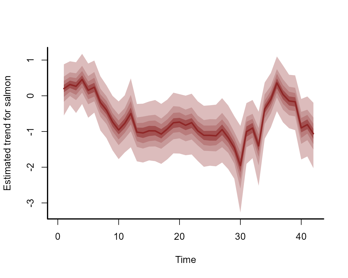

plot(mod1, type = 'forecast')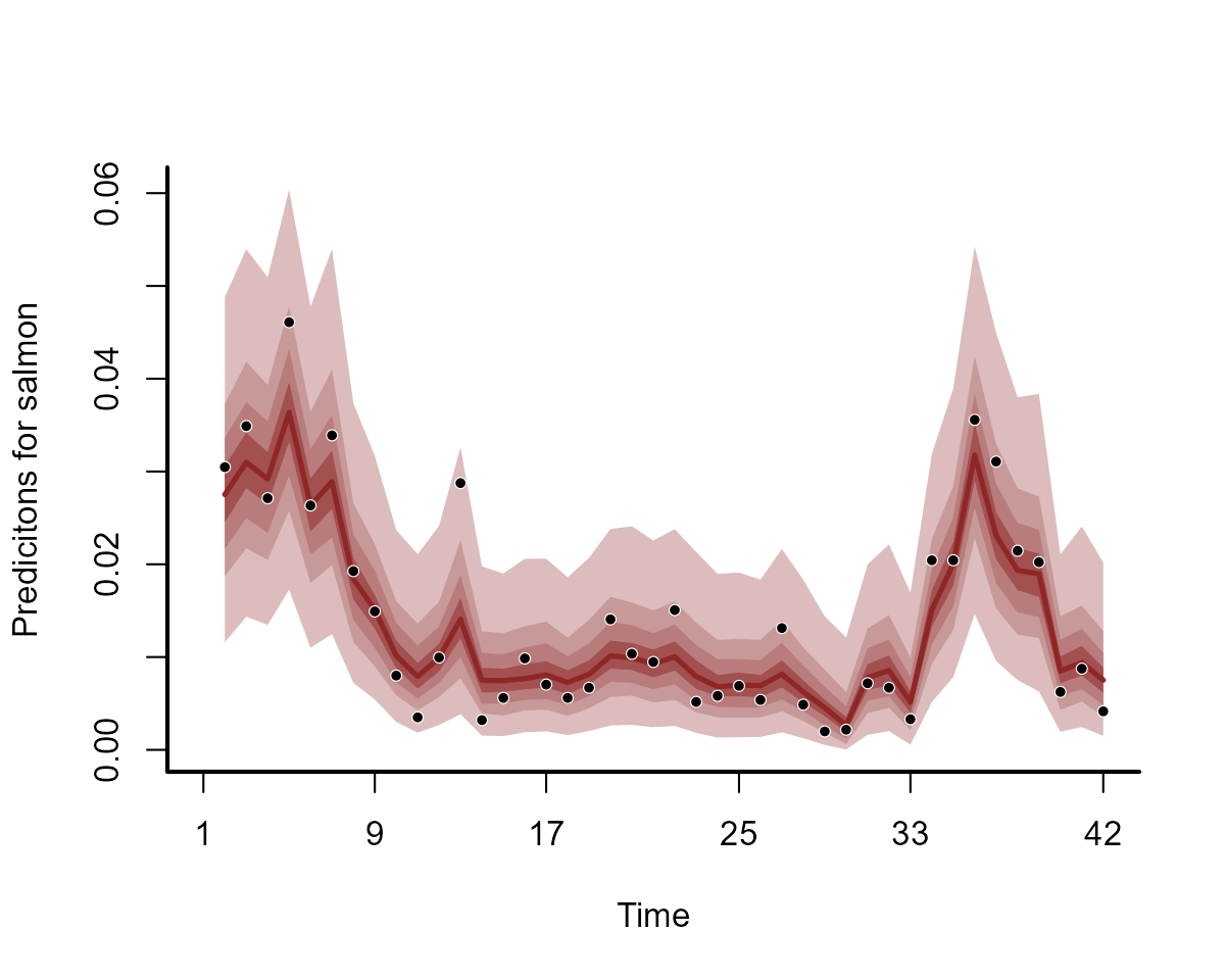

But the process error parameter \(\sigma\) is slightly smaller for this model than for the first model:

# Extract estimates of the process error 'sigma' for each model
mod0_sigma <- as.data.frame(mod0, variable = 'sigma', regex = TRUE) %>%
  dplyr::mutate(model = 'Mod0')
mod1_sigma <- as.data.frame(mod1, variable = 'sigma', regex = TRUE) %>%
  dplyr::mutate(model = 'Mod1')
sigmas <- rbind(mod0_sigma, mod1_sigma)

# Plot using ggplot2
library(ggplot2)
ggplot(sigmas, aes(y = `sigma[1]`, fill = model)) +
  geom_density(alpha = 0.3, colour = NA) +
  coord_flip()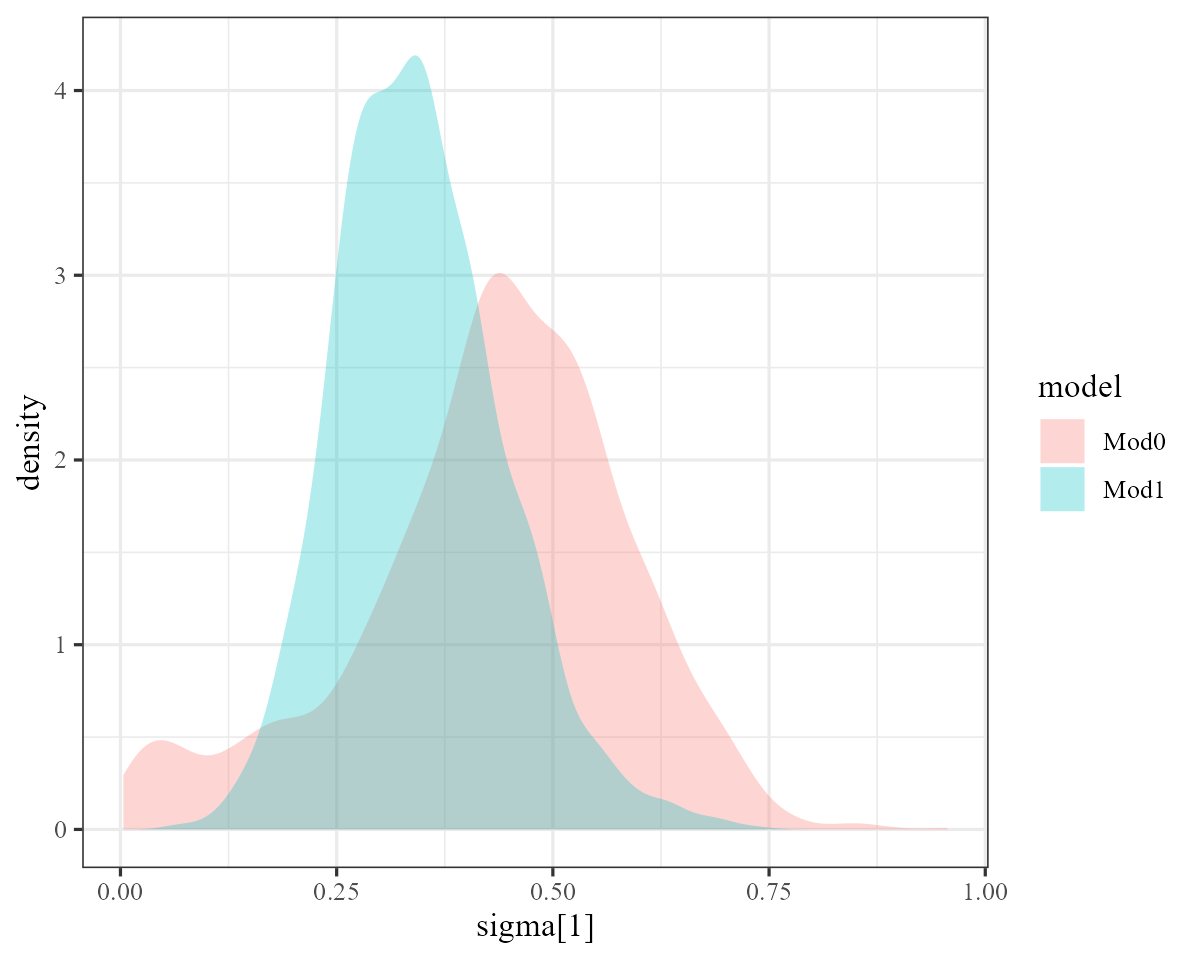

Why does the process error not need to be as flexible in the second model? Because the estimates of this dynamic process are now informed partly by the time-varying effect of upwelling, which we can visualise on the link scale using plot() with trend_effects = TRUE:

plot(mod1, type = 'smooth', trend_effects = TRUE)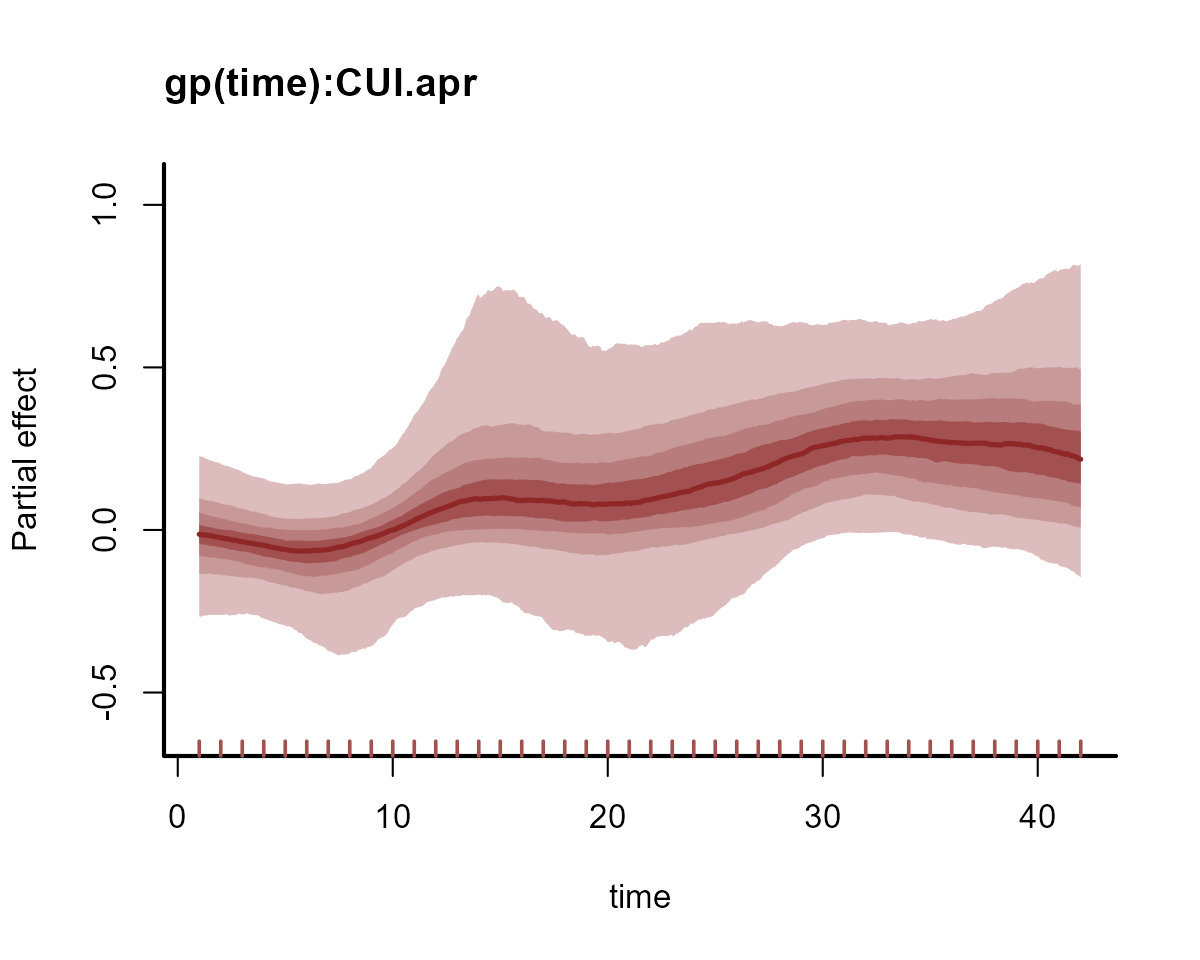

Or on the outcome scale, at a range of possible CUI.apr values, using plot_predictions():

plot_predictions(mod1, newdata = datagrid(CUI.apr = range_round,
                                          time = unique),
                 by = c('time', 'CUI.apr', 'CUI.apr'))

Comparing model predictive performances

A key question when fitting multiple time series models is whether one of them provides better predictions than the other. There are several options in mvgam for exploring this quantitatively. First, we can compare models based on in-sample approximate leave-one-out cross-validation as implemented in the popular loo package:

loo_compare(mod0, mod1)

## Warning: Some Pareto k diagnostic values are too high. See help('pareto-k-diagnostic') for details.

## Warning: Some Pareto k diagnostic values are too high. See help('pareto-k-diagnostic') for details.

##      elpd_diff se_diff
## mod1  0.0       0.0   
## mod0 -2.3       1.6

The second model has the larger Expected Log Predictive Density (ELPD), meaning that it is slightly favoured over the simpler model that did not include the time-varying upwelling effect. However, the two models certainly do not differ by much. But this metric only compares in-sample performance, and we are hoping to use our models to produce reasonable forecasts. Luckily, mvgam also has routines for comparing models using approximate leave-future-out cross-validation. Here we refit both models to a reduced training set (starting at time point 30) and produce approximate 1-step ahead forecasts. These forecasts are used to estimate forecast ELPD before expanding the training set one time point at a time. We use Pareto-smoothed importance sampling to reweight posterior predictions, acting as a kind of particle filter so that we don’t need to refit the model too often (you can read more about how this process works in Bürkner et al. 2020).

lfo_mod0 <- lfo_cv(mod0, min_t = 30)
lfo_mod1 <- lfo_cv(mod1, min_t = 30)

The model with the time-varying upwelling effect tends to provides better 1-step ahead forecasts, with a higher total forecast ELPD

sum(lfo_mod0$elpds)

## [1] 35.11835

sum(lfo_mod1$elpds)

## [1] 36.77461

We can also plot the ELPDs for each model as a contrast. Here, values less than zero suggest the time-varying predictor model (Mod1) gives better 1-step ahead forecasts:

plot(x = 1:length(lfo_mod0$elpds) + 30,
     y = lfo_mod0$elpds - lfo_mod1$elpds,
     ylab = 'ELPDmod0 - ELPDmod1',
     xlab = 'Evaluation time point',
     pch = 16,
     col = 'darkred',
     bty = 'l')
abline(h = 0, lty = 'dashed')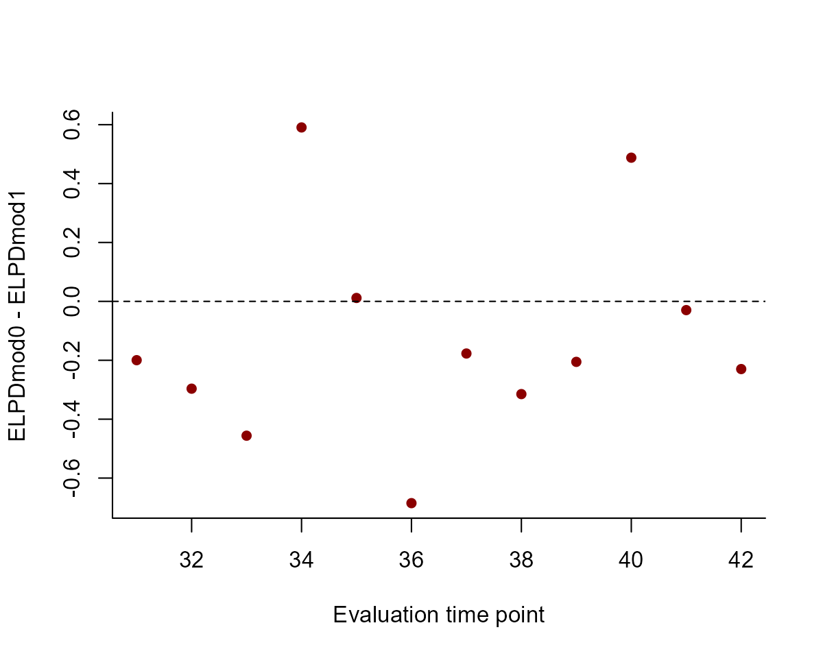

Comparing forecast skill for dynamic beta regression models in mvgam and R

A useful exercise to further expand this model would be to think about what kinds of predictors might impact measurement error, which could easily be implemented into the observation formula in mvgam. But for now, we will leave the model as-is.

Interested in contributing?

I’m actively seeking PhD students and other researchers to work in the areas of ecological forecasting, multivariate model evaluation and development of mvgam. Please reach out if you are interested (n.clark’at’uq.edu.au)

Nicholas J Clark

2024-03-25