Extract the LOOIC (leave-one-out information criterion) using loo::loo().
Usage
# S3 method for mvgam
loo(x, incl_dynamics = FALSE, ...)

# S3 method for mvgam
loo_compare(x, ..., model_names = NULL, incl_dynamics = FALSE)
Arguments
- x
Object of class
mvgam- incl_dynamics
Deprecated and currently ignored
- ...
More
mvgamobjects- model_names
If
NULL(the default) will use model names derived from deparsing the call. Otherwise will use the passed values as model names
Value
For loo.mvgam, an object of class psis_loo (see loo::loo()
for details). For loo_compare.mvgam, an object of class compare.loo
(see loo::loo_compare() for details).
Details
When comparing two (or more) fitted mvgam models, we can estimate the
difference in their in-sample predictive accuracies using the Expected Log
Predictive Density (ELPD). This metric can be approximated using Pareto
Smoothed Importance Sampling (PSIS), which re-weights posterior draws to
approximate predictions for a datapoint had it not been included in the
original model fit (i.e. leave-one-out cross-validation).
See loo::loo() and loo::loo_compare() for further details on how this
importance sampling works.
Note: In-sample predictive metrics such as PSIS-LOO can sometimes be overly
optimistic for models that include process error components (e.g. those with
trend_model, trend_formula, or factor_formula). Consider using
out-of-sample evaluations for further scrutiny (see
forecast.mvgam, score.mvgam_forecast,
lfo_cv).
Examples
# \dontrun{
#--------------------------------------------------
# Simulate 4 time series with hierarchical seasonality
# and independent AR1 dynamic processes
#--------------------------------------------------
set.seed(111)
simdat <- sim_mvgam(
seasonality = 'hierarchical',
trend_model = AR(),
family = gaussian()
)
# Fit a model with shared seasonality
mod1 <- mvgam(
y ~ s(season, bs = 'cc', k = 6),
data = rbind(simdat$data_train, simdat$data_test),
family = gaussian(),
chains = 2,
silent = 2
)
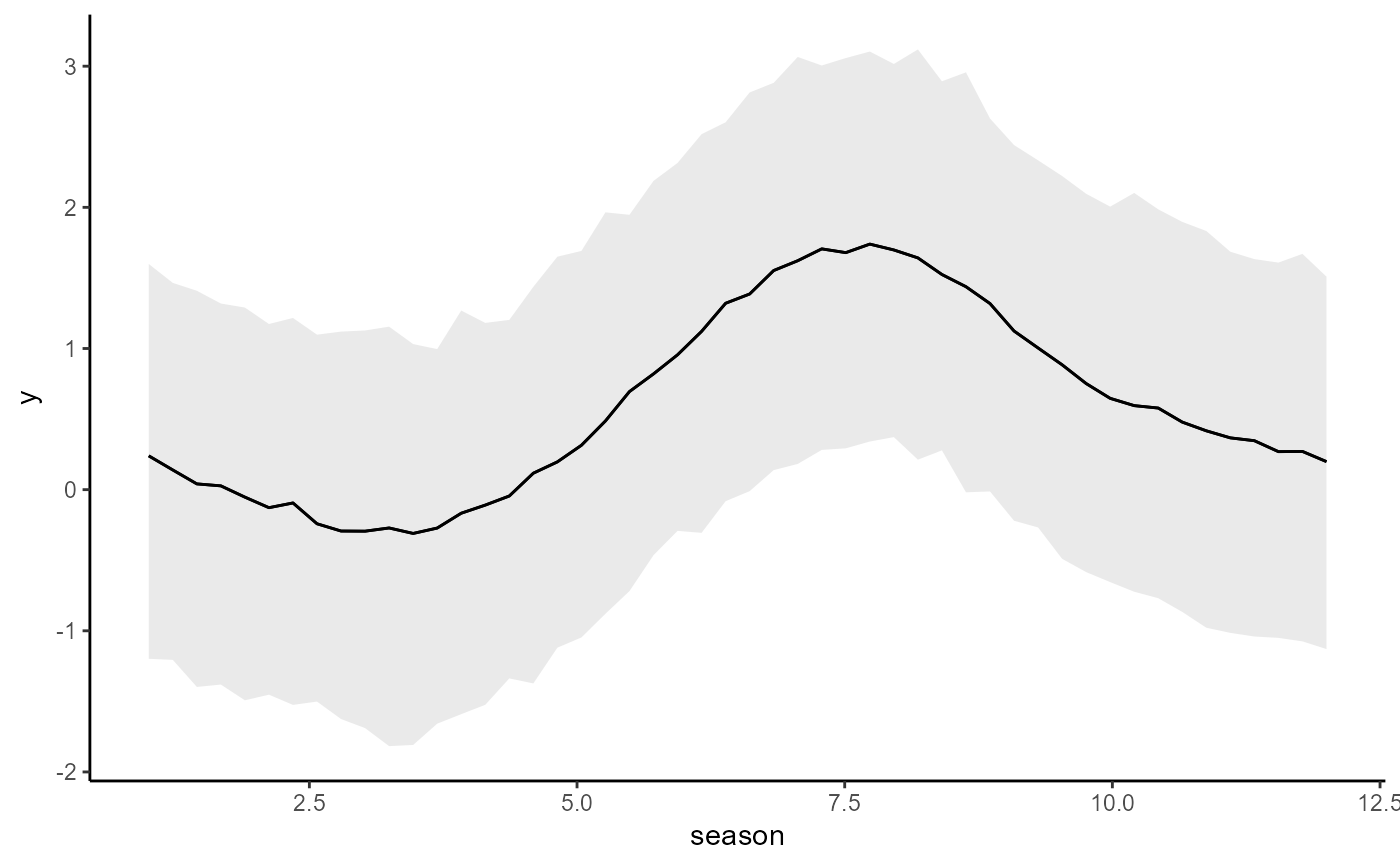
conditional_effects(mod1)
 mc.cores.def <- getOption('mc.cores')
options(mc.cores = 1)
loo(mod1)
#>
#> Computed from 1000 by 300 log-likelihood matrix.
#>
#> Estimate SE
#> elpd_loo -364.2 11.3
#> p_loo 7.6 0.6
#> looic 728.4 22.5
#> ------
#> MCSE of elpd_loo is 0.1.
#> MCSE and ESS estimates assume MCMC draws (r_eff in [0.8, 1.9]).
#>
#> All Pareto k estimates are good (k < 0.67).
#> See help('pareto-k-diagnostic') for details.
# Fit a model with hierarchical seasonality
mod2 <- update(
mod1,
formula = y ~ s(season, bs = 'cc', k = 6) +
s(season, series, bs = 'fs', xt = list(bs = 'cc'), k = 4),
chains = 2,
silent = 2
)
#> Warning: model has repeated 1-d smooths of same variable.
#> Warning: model has repeated 1-d smooths of same variable.
#> Warning: model has repeated 1-d smooths of same variable.
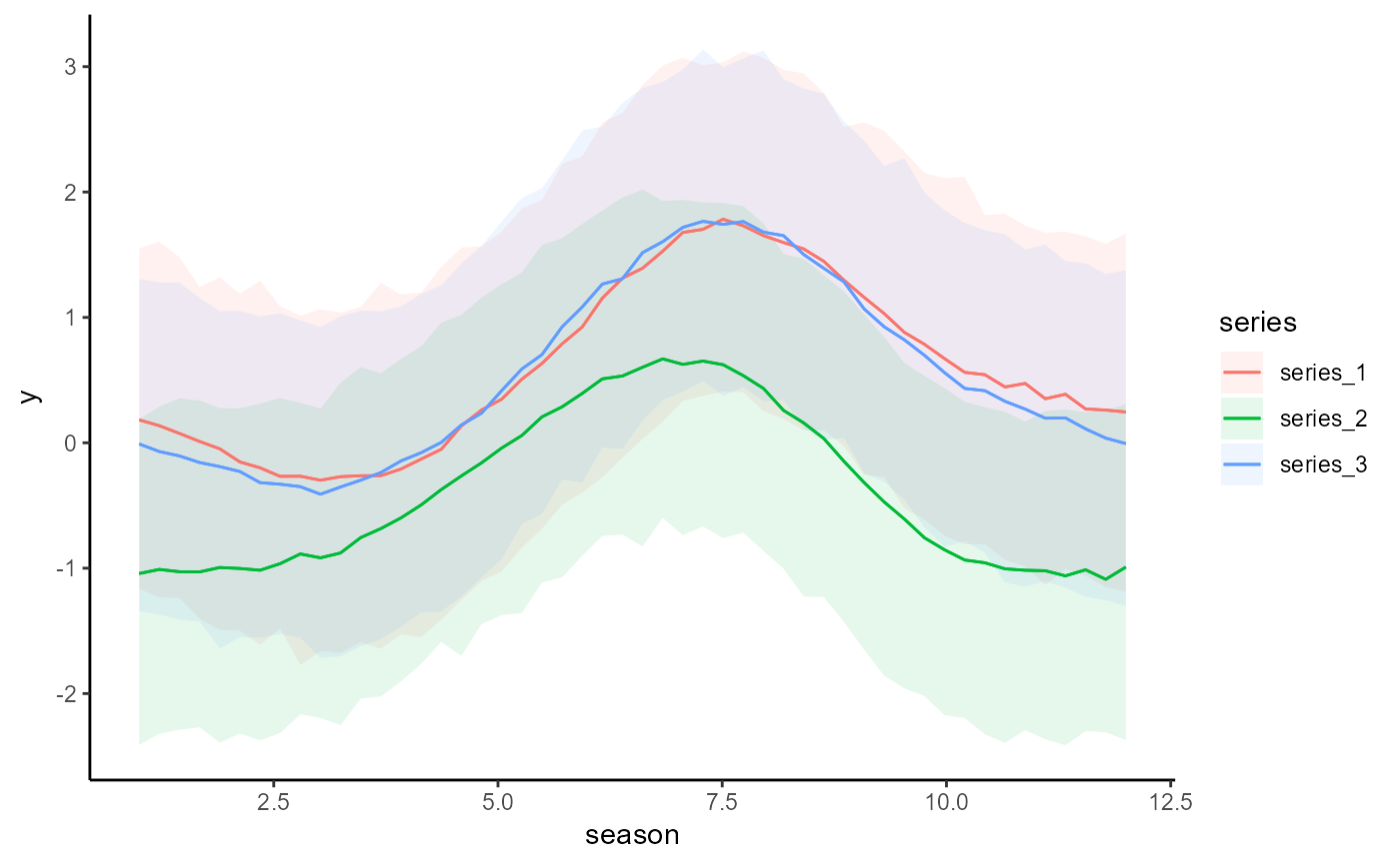
conditional_effects(mod2)
mc.cores.def <- getOption('mc.cores')
options(mc.cores = 1)
loo(mod1)
#>
#> Computed from 1000 by 300 log-likelihood matrix.
#>
#> Estimate SE
#> elpd_loo -364.2 11.3
#> p_loo 7.6 0.6
#> looic 728.4 22.5
#> ------
#> MCSE of elpd_loo is 0.1.
#> MCSE and ESS estimates assume MCMC draws (r_eff in [0.8, 1.9]).
#>
#> All Pareto k estimates are good (k < 0.67).
#> See help('pareto-k-diagnostic') for details.
# Fit a model with hierarchical seasonality
mod2 <- update(
mod1,
formula = y ~ s(season, bs = 'cc', k = 6) +
s(season, series, bs = 'fs', xt = list(bs = 'cc'), k = 4),
chains = 2,
silent = 2
)
#> Warning: model has repeated 1-d smooths of same variable.
#> Warning: model has repeated 1-d smooths of same variable.
#> Warning: model has repeated 1-d smooths of same variable.
conditional_effects(mod2)
 loo(mod2)
#>
#> Computed from 1000 by 300 log-likelihood matrix.
#>
#> Estimate SE
#> elpd_loo -309.5 11.5
#> p_loo 13.3 1.1
#> looic 619.1 23.1
#> ------
#> MCSE of elpd_loo is 0.1.
#> MCSE and ESS estimates assume MCMC draws (r_eff in [0.6, 1.5]).
#>
#> All Pareto k estimates are good (k < 0.67).
#> See help('pareto-k-diagnostic') for details.
# Add AR1 dynamic errors to mod2
mod3 <- update(
mod2,
trend_model = AR(),
chains = 2,
silent = 2
)
#> Warning: model has repeated 1-d smooths of same variable.
#> Warning: model has repeated 1-d smooths of same variable.
#> Warning: model has repeated 1-d smooths of same variable.
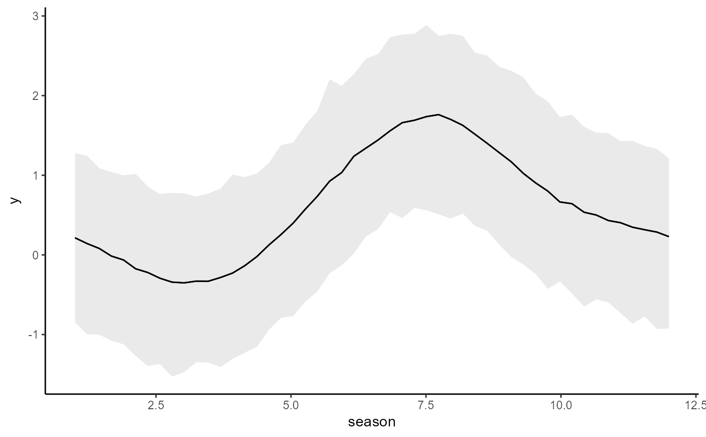
conditional_effects(mod3)
loo(mod2)
#>
#> Computed from 1000 by 300 log-likelihood matrix.
#>
#> Estimate SE
#> elpd_loo -309.5 11.5
#> p_loo 13.3 1.1
#> looic 619.1 23.1
#> ------
#> MCSE of elpd_loo is 0.1.
#> MCSE and ESS estimates assume MCMC draws (r_eff in [0.6, 1.5]).
#>
#> All Pareto k estimates are good (k < 0.67).
#> See help('pareto-k-diagnostic') for details.
# Add AR1 dynamic errors to mod2
mod3 <- update(
mod2,
trend_model = AR(),
chains = 2,
silent = 2
)
#> Warning: model has repeated 1-d smooths of same variable.
#> Warning: model has repeated 1-d smooths of same variable.
#> Warning: model has repeated 1-d smooths of same variable.
conditional_effects(mod3)
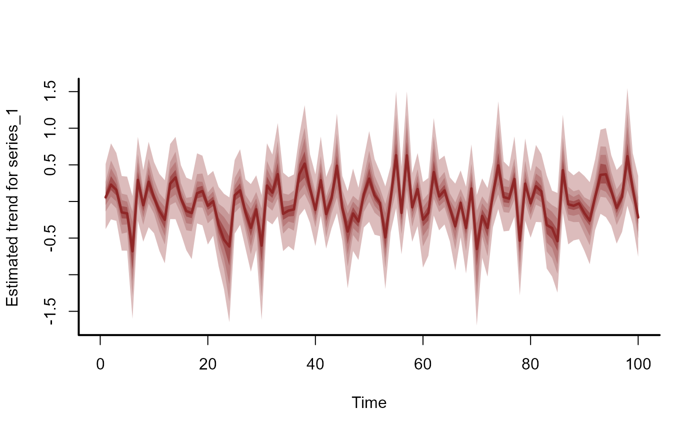
 plot(mod3, type = 'trend')
 loo(mod3)
#> Warning: Some Pareto k diagnostic values are too high. See help('pareto-k-diagnostic') for details.
#>
#> Computed from 1000 by 300 log-likelihood matrix.
#>
#> Estimate SE
#> elpd_loo -243.4 10.2
#> p_loo 180.6 7.7
#> looic 486.8 20.5
#> ------
#> MCSE of elpd_loo is NA.
#> MCSE and ESS estimates assume MCMC draws (r_eff in [0.0, 0.1]).
#>
#> Pareto k diagnostic values:
#> Count Pct. Min. ESS
#> (-Inf, 0.67] (good) 141 47.0% 1
#> (0.67, 1] (bad) 149 49.7% <NA>
#> (1, Inf) (very bad) 10 3.3% <NA>
#> See help('pareto-k-diagnostic') for details.
#--------------------------------------------------
# Compare models using LOO
#--------------------------------------------------
loo_compare(mod1, mod2, mod3)
#> Warning: Some Pareto k diagnostic values are too high. See help('pareto-k-diagnostic') for details.
#> elpd_diff se_diff
#> mod3 0.0 0.0
#> mod2 -66.1 5.5
#> mod1 -120.8 9.8
options(mc.cores = mc.cores.def)
#--------------------------------------------------
# Compare forecast abilities using LFO-CV
#--------------------------------------------------
lfo_mod2 <- lfo_cv(mod2, min_t = 92)
#> Warning: model has repeated 1-d smooths of same variable.
#> Warning: model has repeated 1-d smooths of same variable.
#> Warning: model has repeated 1-d smooths of same variable.
#> Compiling Stan program using cmdstanr
#>
#> Start sampling
#> Running MCMC with 2 parallel chains...
#>
#> Chain 1 Iteration: 1 / 1000 [ 0%] (Warmup)
#> Chain 1 Iteration: 100 / 1000 [ 10%] (Warmup)
#> Chain 2 Iteration: 1 / 1000 [ 0%] (Warmup)
#> Chain 2 Iteration: 100 / 1000 [ 10%] (Warmup)
#> Chain 1 Iteration: 200 / 1000 [ 20%] (Warmup)
#> Chain 2 Iteration: 200 / 1000 [ 20%] (Warmup)
#> Chain 1 Iteration: 300 / 1000 [ 30%] (Warmup)
#> Chain 2 Iteration: 300 / 1000 [ 30%] (Warmup)
#> Chain 1 Iteration: 400 / 1000 [ 40%] (Warmup)
#> Chain 2 Iteration: 400 / 1000 [ 40%] (Warmup)
#> Chain 1 Iteration: 500 / 1000 [ 50%] (Warmup)
#> Chain 1 Iteration: 501 / 1000 [ 50%] (Sampling)
#> Chain 2 Iteration: 500 / 1000 [ 50%] (Warmup)
#> Chain 2 Iteration: 501 / 1000 [ 50%] (Sampling)
#> Chain 1 Iteration: 600 / 1000 [ 60%] (Sampling)
#> Chain 2 Iteration: 600 / 1000 [ 60%] (Sampling)
#> Chain 1 Iteration: 700 / 1000 [ 70%] (Sampling)
#> Chain 1 Iteration: 800 / 1000 [ 80%] (Sampling)
#> Chain 2 Iteration: 700 / 1000 [ 70%] (Sampling)
#> Chain 1 Iteration: 900 / 1000 [ 90%] (Sampling)
#> Chain 2 Iteration: 800 / 1000 [ 80%] (Sampling)
#> Chain 1 Iteration: 1000 / 1000 [100%] (Sampling)
#> Chain 2 Iteration: 900 / 1000 [ 90%] (Sampling)
#> Chain 1 finished in 1.3 seconds.
#> Chain 2 Iteration: 1000 / 1000 [100%] (Sampling)
#> Chain 2 finished in 1.4 seconds.
#>
#> Both chains finished successfully.
#> Mean chain execution time: 1.3 seconds.
#> Total execution time: 1.6 seconds.
#>
lfo_mod3 <- lfo_cv(mod3, min_t = 92)
#> Warning: model has repeated 1-d smooths of same variable.
#> Warning: model has repeated 1-d smooths of same variable.
#> Warning: model has repeated 1-d smooths of same variable.
#> Your model may benefit from using "noncentred = TRUE"
#> Compiling Stan program using cmdstanr
#>
#> Start sampling
#> Running MCMC with 2 parallel chains...
#>
#> Chain 1 Iteration: 1 / 1000 [ 0%] (Warmup)
#> Chain 2 Iteration: 1 / 1000 [ 0%] (Warmup)
#> Chain 2 Iteration: 100 / 1000 [ 10%] (Warmup)
#> Chain 1 Iteration: 100 / 1000 [ 10%] (Warmup)
#> Chain 2 Iteration: 200 / 1000 [ 20%] (Warmup)
#> Chain 1 Iteration: 200 / 1000 [ 20%] (Warmup)
#> Chain 1 Iteration: 300 / 1000 [ 30%] (Warmup)
#> Chain 2 Iteration: 300 / 1000 [ 30%] (Warmup)
#> Chain 1 Iteration: 400 / 1000 [ 40%] (Warmup)
#> Chain 2 Iteration: 400 / 1000 [ 40%] (Warmup)
#> Chain 1 Iteration: 500 / 1000 [ 50%] (Warmup)
#> Chain 1 Iteration: 501 / 1000 [ 50%] (Sampling)
#> Chain 2 Iteration: 500 / 1000 [ 50%] (Warmup)
#> Chain 2 Iteration: 501 / 1000 [ 50%] (Sampling)
#> Chain 1 Iteration: 600 / 1000 [ 60%] (Sampling)
#> Chain 2 Iteration: 600 / 1000 [ 60%] (Sampling)
#> Chain 2 Iteration: 700 / 1000 [ 70%] (Sampling)
#> Chain 1 Iteration: 700 / 1000 [ 70%] (Sampling)
#> Chain 2 Iteration: 800 / 1000 [ 80%] (Sampling)
#> Chain 2 Iteration: 900 / 1000 [ 90%] (Sampling)
#> Chain 1 Iteration: 800 / 1000 [ 80%] (Sampling)
#> Chain 2 Iteration: 1000 / 1000 [100%] (Sampling)
#> Chain 2 finished in 14.1 seconds.
#> Chain 1 Iteration: 900 / 1000 [ 90%] (Sampling)
#> Chain 1 Iteration: 1000 / 1000 [100%] (Sampling)
#> Chain 1 finished in 17.5 seconds.
#>
#> Both chains finished successfully.
#> Mean chain execution time: 15.8 seconds.
#> Total execution time: 17.6 seconds.
#>
#> Warning: model has repeated 1-d smooths of same variable.
#> Warning: model has repeated 1-d smooths of same variable.
#> Warning: model has repeated 1-d smooths of same variable.
#> Your model may benefit from using "noncentred = TRUE"
#> Compiling Stan program using cmdstanr
#>
#> Start sampling
#> Running MCMC with 2 parallel chains...
#>
#> Chain 1 Iteration: 1 / 1000 [ 0%] (Warmup)
#> Chain 2 Iteration: 1 / 1000 [ 0%] (Warmup)
#> Chain 1 Iteration: 100 / 1000 [ 10%] (Warmup)
#> Chain 2 Iteration: 100 / 1000 [ 10%] (Warmup)
#> Chain 1 Iteration: 200 / 1000 [ 20%] (Warmup)
#> Chain 1 Iteration: 300 / 1000 [ 30%] (Warmup)
#> Chain 2 Iteration: 200 / 1000 [ 20%] (Warmup)
#> Chain 1 Iteration: 400 / 1000 [ 40%] (Warmup)
#> Chain 1 Iteration: 500 / 1000 [ 50%] (Warmup)
#> Chain 1 Iteration: 501 / 1000 [ 50%] (Sampling)
#> Chain 1 Iteration: 600 / 1000 [ 60%] (Sampling)
#> Chain 2 Iteration: 300 / 1000 [ 30%] (Warmup)
#> Chain 1 Iteration: 700 / 1000 [ 70%] (Sampling)
#> Chain 1 Iteration: 800 / 1000 [ 80%] (Sampling)
#> Chain 2 Iteration: 400 / 1000 [ 40%] (Warmup)
#> Chain 1 Iteration: 900 / 1000 [ 90%] (Sampling)
#> Chain 1 Iteration: 1000 / 1000 [100%] (Sampling)
#> Chain 1 finished in 14.6 seconds.
#> Chain 2 Iteration: 500 / 1000 [ 50%] (Warmup)
#> Chain 2 Iteration: 501 / 1000 [ 50%] (Sampling)
#> Chain 2 Iteration: 600 / 1000 [ 60%] (Sampling)
#> Chain 2 Iteration: 700 / 1000 [ 70%] (Sampling)
#> Chain 2 Iteration: 800 / 1000 [ 80%] (Sampling)
#> Chain 2 Iteration: 900 / 1000 [ 90%] (Sampling)
#> Chain 2 Iteration: 1000 / 1000 [100%] (Sampling)
#> Chain 2 finished in 25.6 seconds.
#>
#> Both chains finished successfully.
#> Mean chain execution time: 20.1 seconds.
#> Total execution time: 25.8 seconds.
#>
#> Warning: model has repeated 1-d smooths of same variable.
#> Warning: model has repeated 1-d smooths of same variable.
#> Warning: model has repeated 1-d smooths of same variable.
#> Your model may benefit from using "noncentred = TRUE"
#> Compiling Stan program using cmdstanr
#>
#> Start sampling
#> Running MCMC with 2 parallel chains...
#>
#> Chain 1 Iteration: 1 / 1000 [ 0%] (Warmup)
#> Chain 2 Iteration: 1 / 1000 [ 0%] (Warmup)
#> Chain 1 Iteration: 100 / 1000 [ 10%] (Warmup)
#> Chain 2 Iteration: 100 / 1000 [ 10%] (Warmup)
#> Chain 1 Iteration: 200 / 1000 [ 20%] (Warmup)
#> Chain 2 Iteration: 200 / 1000 [ 20%] (Warmup)
#> Chain 1 Iteration: 300 / 1000 [ 30%] (Warmup)
#> Chain 2 Iteration: 300 / 1000 [ 30%] (Warmup)
#> Chain 1 Iteration: 400 / 1000 [ 40%] (Warmup)
#> Chain 2 Iteration: 400 / 1000 [ 40%] (Warmup)
#> Chain 1 Iteration: 500 / 1000 [ 50%] (Warmup)
#> Chain 1 Iteration: 501 / 1000 [ 50%] (Sampling)
#> Chain 2 Iteration: 500 / 1000 [ 50%] (Warmup)
#> Chain 2 Iteration: 501 / 1000 [ 50%] (Sampling)
#> Chain 1 Iteration: 600 / 1000 [ 60%] (Sampling)
#> Chain 2 Iteration: 600 / 1000 [ 60%] (Sampling)
#> Chain 1 Iteration: 700 / 1000 [ 70%] (Sampling)
#> Chain 2 Iteration: 700 / 1000 [ 70%] (Sampling)
#> Chain 1 Iteration: 800 / 1000 [ 80%] (Sampling)
#> Chain 2 Iteration: 800 / 1000 [ 80%] (Sampling)
#> Chain 1 Iteration: 900 / 1000 [ 90%] (Sampling)
#> Chain 2 Iteration: 900 / 1000 [ 90%] (Sampling)
#> Chain 1 Iteration: 1000 / 1000 [100%] (Sampling)
#> Chain 1 finished in 23.1 seconds.
#> Chain 2 Iteration: 1000 / 1000 [100%] (Sampling)
#> Chain 2 finished in 24.8 seconds.
#>
#> Both chains finished successfully.
#> Mean chain execution time: 23.9 seconds.
#> Total execution time: 25.0 seconds.
#>
# Plot forecast ELPD differences
plot(
y = lfo_mod2$elpds - lfo_mod3$elpds,
x = lfo_mod2$eval_timepoints,
pch = 16,
ylab = 'ELPD_mod2 - ELPD_mod3',
xlab = 'Evaluation timepoint'
)
abline(h = 0, lty = 'dashed')
loo(mod3)
#> Warning: Some Pareto k diagnostic values are too high. See help('pareto-k-diagnostic') for details.
#>
#> Computed from 1000 by 300 log-likelihood matrix.
#>
#> Estimate SE
#> elpd_loo -243.4 10.2
#> p_loo 180.6 7.7
#> looic 486.8 20.5
#> ------
#> MCSE of elpd_loo is NA.
#> MCSE and ESS estimates assume MCMC draws (r_eff in [0.0, 0.1]).
#>
#> Pareto k diagnostic values:
#> Count Pct. Min. ESS
#> (-Inf, 0.67] (good) 141 47.0% 1
#> (0.67, 1] (bad) 149 49.7% <NA>
#> (1, Inf) (very bad) 10 3.3% <NA>
#> See help('pareto-k-diagnostic') for details.
#--------------------------------------------------
# Compare models using LOO
#--------------------------------------------------
loo_compare(mod1, mod2, mod3)
#> Warning: Some Pareto k diagnostic values are too high. See help('pareto-k-diagnostic') for details.
#> elpd_diff se_diff
#> mod3 0.0 0.0
#> mod2 -66.1 5.5
#> mod1 -120.8 9.8
options(mc.cores = mc.cores.def)
#--------------------------------------------------
# Compare forecast abilities using LFO-CV
#--------------------------------------------------
lfo_mod2 <- lfo_cv(mod2, min_t = 92)
#> Warning: model has repeated 1-d smooths of same variable.
#> Warning: model has repeated 1-d smooths of same variable.
#> Warning: model has repeated 1-d smooths of same variable.
#> Compiling Stan program using cmdstanr
#>
#> Start sampling
#> Running MCMC with 2 parallel chains...
#>
#> Chain 1 Iteration: 1 / 1000 [ 0%] (Warmup)
#> Chain 1 Iteration: 100 / 1000 [ 10%] (Warmup)
#> Chain 2 Iteration: 1 / 1000 [ 0%] (Warmup)
#> Chain 2 Iteration: 100 / 1000 [ 10%] (Warmup)
#> Chain 1 Iteration: 200 / 1000 [ 20%] (Warmup)
#> Chain 2 Iteration: 200 / 1000 [ 20%] (Warmup)
#> Chain 1 Iteration: 300 / 1000 [ 30%] (Warmup)
#> Chain 2 Iteration: 300 / 1000 [ 30%] (Warmup)
#> Chain 1 Iteration: 400 / 1000 [ 40%] (Warmup)
#> Chain 2 Iteration: 400 / 1000 [ 40%] (Warmup)
#> Chain 1 Iteration: 500 / 1000 [ 50%] (Warmup)
#> Chain 1 Iteration: 501 / 1000 [ 50%] (Sampling)
#> Chain 2 Iteration: 500 / 1000 [ 50%] (Warmup)
#> Chain 2 Iteration: 501 / 1000 [ 50%] (Sampling)
#> Chain 1 Iteration: 600 / 1000 [ 60%] (Sampling)
#> Chain 2 Iteration: 600 / 1000 [ 60%] (Sampling)
#> Chain 1 Iteration: 700 / 1000 [ 70%] (Sampling)
#> Chain 1 Iteration: 800 / 1000 [ 80%] (Sampling)
#> Chain 2 Iteration: 700 / 1000 [ 70%] (Sampling)
#> Chain 1 Iteration: 900 / 1000 [ 90%] (Sampling)
#> Chain 2 Iteration: 800 / 1000 [ 80%] (Sampling)
#> Chain 1 Iteration: 1000 / 1000 [100%] (Sampling)
#> Chain 2 Iteration: 900 / 1000 [ 90%] (Sampling)
#> Chain 1 finished in 1.3 seconds.
#> Chain 2 Iteration: 1000 / 1000 [100%] (Sampling)
#> Chain 2 finished in 1.4 seconds.
#>
#> Both chains finished successfully.
#> Mean chain execution time: 1.3 seconds.
#> Total execution time: 1.6 seconds.
#>
lfo_mod3 <- lfo_cv(mod3, min_t = 92)
#> Warning: model has repeated 1-d smooths of same variable.
#> Warning: model has repeated 1-d smooths of same variable.
#> Warning: model has repeated 1-d smooths of same variable.
#> Your model may benefit from using "noncentred = TRUE"
#> Compiling Stan program using cmdstanr
#>
#> Start sampling
#> Running MCMC with 2 parallel chains...
#>
#> Chain 1 Iteration: 1 / 1000 [ 0%] (Warmup)
#> Chain 2 Iteration: 1 / 1000 [ 0%] (Warmup)
#> Chain 2 Iteration: 100 / 1000 [ 10%] (Warmup)
#> Chain 1 Iteration: 100 / 1000 [ 10%] (Warmup)
#> Chain 2 Iteration: 200 / 1000 [ 20%] (Warmup)
#> Chain 1 Iteration: 200 / 1000 [ 20%] (Warmup)
#> Chain 1 Iteration: 300 / 1000 [ 30%] (Warmup)
#> Chain 2 Iteration: 300 / 1000 [ 30%] (Warmup)
#> Chain 1 Iteration: 400 / 1000 [ 40%] (Warmup)
#> Chain 2 Iteration: 400 / 1000 [ 40%] (Warmup)
#> Chain 1 Iteration: 500 / 1000 [ 50%] (Warmup)
#> Chain 1 Iteration: 501 / 1000 [ 50%] (Sampling)
#> Chain 2 Iteration: 500 / 1000 [ 50%] (Warmup)
#> Chain 2 Iteration: 501 / 1000 [ 50%] (Sampling)
#> Chain 1 Iteration: 600 / 1000 [ 60%] (Sampling)
#> Chain 2 Iteration: 600 / 1000 [ 60%] (Sampling)
#> Chain 2 Iteration: 700 / 1000 [ 70%] (Sampling)
#> Chain 1 Iteration: 700 / 1000 [ 70%] (Sampling)
#> Chain 2 Iteration: 800 / 1000 [ 80%] (Sampling)
#> Chain 2 Iteration: 900 / 1000 [ 90%] (Sampling)
#> Chain 1 Iteration: 800 / 1000 [ 80%] (Sampling)
#> Chain 2 Iteration: 1000 / 1000 [100%] (Sampling)
#> Chain 2 finished in 14.1 seconds.
#> Chain 1 Iteration: 900 / 1000 [ 90%] (Sampling)
#> Chain 1 Iteration: 1000 / 1000 [100%] (Sampling)
#> Chain 1 finished in 17.5 seconds.
#>
#> Both chains finished successfully.
#> Mean chain execution time: 15.8 seconds.
#> Total execution time: 17.6 seconds.
#>
#> Warning: model has repeated 1-d smooths of same variable.
#> Warning: model has repeated 1-d smooths of same variable.
#> Warning: model has repeated 1-d smooths of same variable.
#> Your model may benefit from using "noncentred = TRUE"
#> Compiling Stan program using cmdstanr
#>
#> Start sampling
#> Running MCMC with 2 parallel chains...
#>
#> Chain 1 Iteration: 1 / 1000 [ 0%] (Warmup)
#> Chain 2 Iteration: 1 / 1000 [ 0%] (Warmup)
#> Chain 1 Iteration: 100 / 1000 [ 10%] (Warmup)
#> Chain 2 Iteration: 100 / 1000 [ 10%] (Warmup)
#> Chain 1 Iteration: 200 / 1000 [ 20%] (Warmup)
#> Chain 1 Iteration: 300 / 1000 [ 30%] (Warmup)
#> Chain 2 Iteration: 200 / 1000 [ 20%] (Warmup)
#> Chain 1 Iteration: 400 / 1000 [ 40%] (Warmup)
#> Chain 1 Iteration: 500 / 1000 [ 50%] (Warmup)
#> Chain 1 Iteration: 501 / 1000 [ 50%] (Sampling)
#> Chain 1 Iteration: 600 / 1000 [ 60%] (Sampling)
#> Chain 2 Iteration: 300 / 1000 [ 30%] (Warmup)
#> Chain 1 Iteration: 700 / 1000 [ 70%] (Sampling)
#> Chain 1 Iteration: 800 / 1000 [ 80%] (Sampling)
#> Chain 2 Iteration: 400 / 1000 [ 40%] (Warmup)
#> Chain 1 Iteration: 900 / 1000 [ 90%] (Sampling)
#> Chain 1 Iteration: 1000 / 1000 [100%] (Sampling)
#> Chain 1 finished in 14.6 seconds.
#> Chain 2 Iteration: 500 / 1000 [ 50%] (Warmup)
#> Chain 2 Iteration: 501 / 1000 [ 50%] (Sampling)
#> Chain 2 Iteration: 600 / 1000 [ 60%] (Sampling)
#> Chain 2 Iteration: 700 / 1000 [ 70%] (Sampling)
#> Chain 2 Iteration: 800 / 1000 [ 80%] (Sampling)
#> Chain 2 Iteration: 900 / 1000 [ 90%] (Sampling)
#> Chain 2 Iteration: 1000 / 1000 [100%] (Sampling)
#> Chain 2 finished in 25.6 seconds.
#>
#> Both chains finished successfully.
#> Mean chain execution time: 20.1 seconds.
#> Total execution time: 25.8 seconds.
#>
#> Warning: model has repeated 1-d smooths of same variable.
#> Warning: model has repeated 1-d smooths of same variable.
#> Warning: model has repeated 1-d smooths of same variable.
#> Your model may benefit from using "noncentred = TRUE"
#> Compiling Stan program using cmdstanr
#>
#> Start sampling
#> Running MCMC with 2 parallel chains...
#>
#> Chain 1 Iteration: 1 / 1000 [ 0%] (Warmup)
#> Chain 2 Iteration: 1 / 1000 [ 0%] (Warmup)
#> Chain 1 Iteration: 100 / 1000 [ 10%] (Warmup)
#> Chain 2 Iteration: 100 / 1000 [ 10%] (Warmup)
#> Chain 1 Iteration: 200 / 1000 [ 20%] (Warmup)
#> Chain 2 Iteration: 200 / 1000 [ 20%] (Warmup)
#> Chain 1 Iteration: 300 / 1000 [ 30%] (Warmup)
#> Chain 2 Iteration: 300 / 1000 [ 30%] (Warmup)
#> Chain 1 Iteration: 400 / 1000 [ 40%] (Warmup)
#> Chain 2 Iteration: 400 / 1000 [ 40%] (Warmup)
#> Chain 1 Iteration: 500 / 1000 [ 50%] (Warmup)
#> Chain 1 Iteration: 501 / 1000 [ 50%] (Sampling)
#> Chain 2 Iteration: 500 / 1000 [ 50%] (Warmup)
#> Chain 2 Iteration: 501 / 1000 [ 50%] (Sampling)
#> Chain 1 Iteration: 600 / 1000 [ 60%] (Sampling)
#> Chain 2 Iteration: 600 / 1000 [ 60%] (Sampling)
#> Chain 1 Iteration: 700 / 1000 [ 70%] (Sampling)
#> Chain 2 Iteration: 700 / 1000 [ 70%] (Sampling)
#> Chain 1 Iteration: 800 / 1000 [ 80%] (Sampling)
#> Chain 2 Iteration: 800 / 1000 [ 80%] (Sampling)
#> Chain 1 Iteration: 900 / 1000 [ 90%] (Sampling)
#> Chain 2 Iteration: 900 / 1000 [ 90%] (Sampling)
#> Chain 1 Iteration: 1000 / 1000 [100%] (Sampling)
#> Chain 1 finished in 23.1 seconds.
#> Chain 2 Iteration: 1000 / 1000 [100%] (Sampling)
#> Chain 2 finished in 24.8 seconds.
#>
#> Both chains finished successfully.
#> Mean chain execution time: 23.9 seconds.
#> Total execution time: 25.0 seconds.
#>
# Plot forecast ELPD differences
plot(
y = lfo_mod2$elpds - lfo_mod3$elpds,
x = lfo_mod2$eval_timepoints,
pch = 16,
ylab = 'ELPD_mod2 - ELPD_mod3',
xlab = 'Evaluation timepoint'
)
abline(h = 0, lty = 'dashed')
 # }
# }