This function simulates sets of time series data for fitting a multivariate GAM that includes shared seasonality and dependence on State-Space latent dynamic factors. Random dependencies among series, i.e. correlations in their long-term trends, are included in the form of correlated loadings on the latent dynamic factors
Arguments
- T
integer. Number of observations (timepoints)- n_series
integer. Number of discrete time series- seasonality
character. Eithershared, meaning that all series share the exact same seasonal pattern, orhierarchical, meaning that there is a global seasonality but each series' pattern can deviate slightly- use_lv
logical. IfTRUE, use dynamic factors to estimate series' latent trends in a reduced dimension format. IfFALSE, estimate independent latent trends for each series- n_lv
integer. Number of latent dynamic factors for generating the series' trends. Defaults to0, meaning that dynamics are estimated independently for each series- trend_model
characterspecifying the time series dynamics for the latent trend. Options are:None(no latent trend component; i.e. the GAM component is all that contributes to the linear predictor, and the observation process is the only source of error; similarly to what is estimated bygam)RW(random walk with possible drift)AR1(with possible drift)AR2(with possible drift)AR3(with possible drift)VAR1(contemporaneously uncorrelated VAR1)VAR1cor(contemporaneously correlated VAR1)GP(Gaussian Process with squared exponential kernel)
See mvgam_trends for more details
- drift
logical, simulate a drift term for each trend- prop_trend
numeric. Relative importance of the trend for each series. Should be between0and1- trend_rel
Deprecated. Use
prop_trendinstead- freq
integer. The seasonal frequency of the series- family
familyspecifying the exponential observation family for the series. Currently supported families are:nb(),poisson(),bernoulli(),tweedie(),gaussian(),betar(),lognormal(),student()andGamma()- phi
vectorof dispersion parameters for the series (i.e.sizefornb()orphiforbetar()). Iflength(phi) < n_series, the first element ofphiwill be replicatedn_seriestimes. Defaults to5fornb()andtweedie();10forbetar()- shape
vectorof shape parameters for the series (i.e.shapeforgamma()). Iflength(shape) < n_series, the first element ofshapewill be replicatedn_seriestimes. Defaults to10- sigma
vectorof scale parameters for the series (i.e.sdforgaussian()orstudent(),log(sd)forlognormal()). Iflength(sigma) < n_series, the first element ofsigmawill be replicatedn_seriestimes. Defaults to0.5forgaussian()andstudent();0.2forlognormal()- nu
vectorof degrees of freedom parameters for the series (i.e.nuforstudent()). Iflength(nu) < n_series, the first element ofnuwill be replicatedn_seriestimes. Defaults to3- mu
vectorof location parameters for the series. Iflength(mu) < n_series, the first element ofmuwill be replicatedn_seriestimes. Defaults to small random values between-0.5and0.5on the link scale- prop_missing
numericstating proportion of observations that are missing. Should be between0and0.8, inclusive- prop_train
numericstating the proportion of data to use for training. Should be between0.2and1
Value
A list object containing outputs needed for
mvgam, including 'data_train' and 'data_test', as well
as some additional information about the simulated seasonality and
trend dependencies
References
Clark, N. J. and Wells, K. (2022). Dynamic generalised additive models (DGAMs) for forecasting discrete ecological time series. Methods in Ecology and Evolution, 13(11), 2388-2404. doi:10.1111/2041-210X.13974
Examples
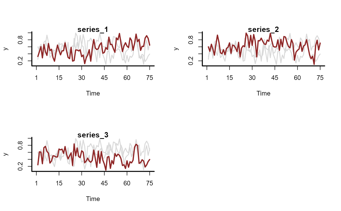
# Simulate series with observations bounded at 0 and 1 (Beta responses)
sim_data <- sim_mvgam(
family = betar(),
trend_model = RW(),
prop_trend = 0.6
)
plot_mvgam_series(data = sim_data$data_train, series = 'all')
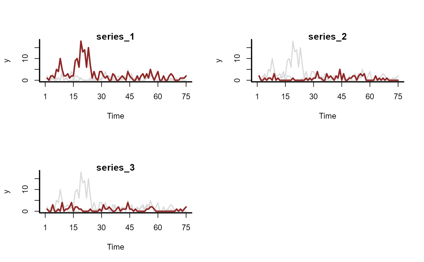
 # Now simulate series with overdispersed discrete observations
sim_data <- sim_mvgam(
family = nb(),
trend_model = RW(),
prop_trend = 0.6,
phi = 10
)
plot_mvgam_series(data = sim_data$data_train, series = 'all')
# Now simulate series with overdispersed discrete observations
sim_data <- sim_mvgam(
family = nb(),
trend_model = RW(),
prop_trend = 0.6,
phi = 10
)
plot_mvgam_series(data = sim_data$data_train, series = 'all')