Extract hindcasts for a fitted mvgam object
Arguments
- object
listobject of classmvgamorjsdgam. Seemvgam()- ...
Ignored
- type
When this has the value
link(default) the linear predictor is calculated on the link scale. Ifexpectedis used, predictions reflect the expectation of the response (the mean) but ignore uncertainty in the observation process. Whenresponseis used, the predictions take uncertainty in the observation process into account to return predictions on the outcome scale. Whenvarianceis used, the variance of the response with respect to the mean (mean-variance relationship) is returned. Whentype = "terms", each component of the linear predictor is returned separately in the form of alist(possibly with standard errors, ifsummary = TRUE): this includes parametric model components, followed by each smooth component, but excludes any offset and any intercept. Two special cases are also allowed: typelatent_Nwill return the estimated latent abundances from an N-mixture distribution, while typedetectionwill return the estimated detection probability from an N-mixture distribution
Value
An object of class mvgam_forecast containing hindcast distributions.
See mvgam_forecast-class for details.
Details
Posterior hindcasts (i.e. retrodictions) are drawn from the fitted mvgam and
organized into a convenient format for plotting
Examples
# \dontrun{
simdat <- sim_mvgam(n_series = 3, trend_model = AR())
mod <- mvgam(y ~ s(season, bs = 'cc'),
trend_model = AR(),
noncentred = TRUE,
data = simdat$data_train,
chains = 2,
silent = 2)
# Hindcasts on response scale
hc <- hindcast(mod)
str(hc)
#> List of 15
#> $ call :Class 'formula' language y ~ s(season, bs = "cc")
#> .. ..- attr(*, ".Environment")=<environment: 0x5582dbecfc90>
#> $ trend_call : NULL
#> $ family : chr "poisson"
#> $ trend_model :List of 7
#> ..$ trend_model: chr "AR1"
#> ..$ ma : logi FALSE
#> ..$ cor : logi FALSE
#> ..$ unit : chr "time"
#> ..$ gr : chr "NA"
#> ..$ subgr : chr "series"
#> ..$ label : language AR()
#> ..- attr(*, "class")= chr "mvgam_trend"
#> ..- attr(*, "param_info")=List of 2
#> .. ..$ param_names: chr [1:8] "trend" "tau" "sigma" "ar1" ...
#> .. ..$ labels : chr [1:8] "trend_estimates" "precision_parameter" "standard_deviation" "autoregressive_coef_1" ...
#> $ drift : logi FALSE
#> $ use_lv : logi FALSE
#> $ fit_engine : chr "stan"
#> $ type : chr "response"
#> $ series_names : chr [1:3] "series_1" "series_2" "series_3"
#> $ train_observations:List of 3
#> ..$ series_1: int [1:75] 2 2 0 0 2 4 6 6 4 1 ...
#> ..$ series_2: int [1:75] 2 1 3 1 0 6 6 3 3 7 ...
#> ..$ series_3: int [1:75] 1 0 0 0 0 1 1 0 1 0 ...
#> $ train_times :List of 3
#> ..$ series_1: int [1:75] 1 2 3 4 5 6 7 8 9 10 ...
#> ..$ series_2: int [1:75] 1 2 3 4 5 6 7 8 9 10 ...
#> ..$ series_3: int [1:75] 1 2 3 4 5 6 7 8 9 10 ...
#> $ test_observations : NULL
#> $ test_times : NULL
#> $ hindcasts :List of 3
#> ..$ series_1: num [1:1000, 1:75] 1 0 0 5 5 2 0 4 1 0 ...
#> .. ..- attr(*, "dimnames")=List of 2
#> .. .. ..$ : NULL
#> .. .. ..$ : chr [1:75] "ypred[1,1]" "ypred[2,1]" "ypred[3,1]" "ypred[4,1]" ...
#> ..$ series_2: num [1:1000, 1:75] 0 2 1 2 1 4 1 2 4 1 ...
#> .. ..- attr(*, "dimnames")=List of 2
#> .. .. ..$ : NULL
#> .. .. ..$ : chr [1:75] "ypred[1,2]" "ypred[2,2]" "ypred[3,2]" "ypred[4,2]" ...
#> ..$ series_3: num [1:1000, 1:75] 0 0 0 0 1 0 0 0 2 0 ...
#> .. ..- attr(*, "dimnames")=List of 2
#> .. .. ..$ : NULL
#> .. .. ..$ : chr [1:75] "ypred[1,3]" "ypred[2,3]" "ypred[3,3]" "ypred[4,3]" ...
#> $ forecasts : NULL
#> - attr(*, "class")= chr "mvgam_forecast"
head(summary(hc), 12)
#> # A tibble: 12 × 7
#> series time predQ50 predQ2.5 predQ97.5 truth type
#> <fct> <int> <dbl> <dbl> <dbl> <int> <chr>
#> 1 series_1 1 1 0 4 2 response
#> 2 series_1 2 0 0 3 2 response
#> 3 series_1 3 0 0 2 0 response
#> 4 series_1 4 0 0 2 0 response
#> 5 series_1 5 1 0 4 2 response
#> 6 series_1 6 3 0 7 4 response
#> 7 series_1 7 4 1 10.0 6 response
#> 8 series_1 8 3 0 9 6 response
#> 9 series_1 9 3 0 8 4 response
#> 10 series_1 10 3 0 8 1 response
#> 11 series_1 11 2 0 6 3 response
#> 12 series_1 12 1 0 4 3 response
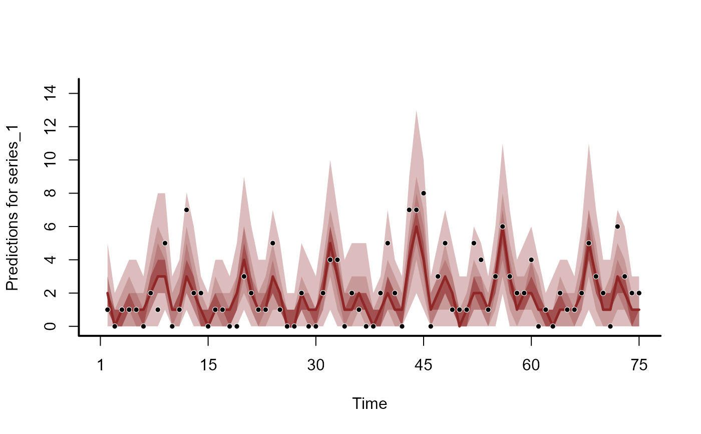
plot(hc, series = 1)
#> No non-missing values in test_observations; cannot calculate forecast score
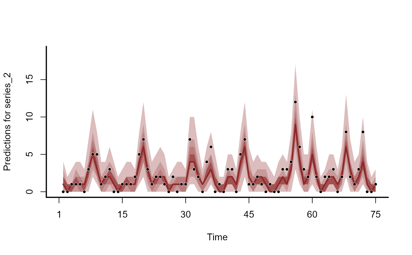
 plot(hc, series = 2)
#> No non-missing values in test_observations; cannot calculate forecast score
plot(hc, series = 2)
#> No non-missing values in test_observations; cannot calculate forecast score
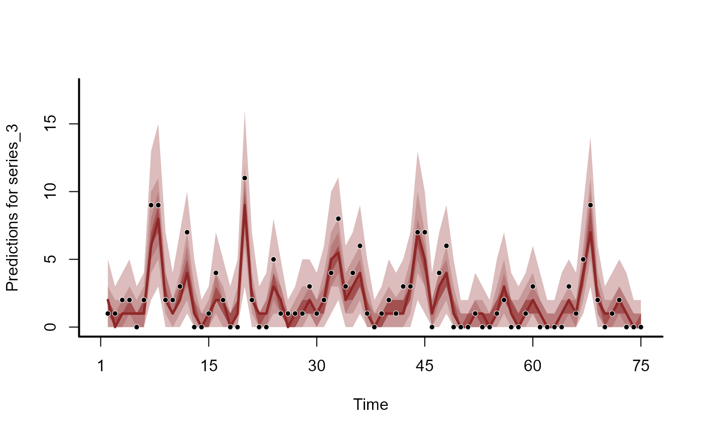
 plot(hc, series = 3)
#> No non-missing values in test_observations; cannot calculate forecast score
plot(hc, series = 3)
#> No non-missing values in test_observations; cannot calculate forecast score
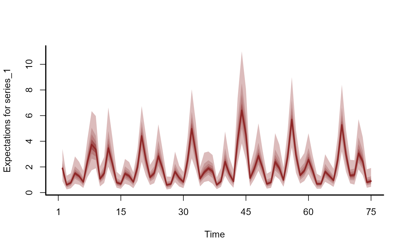
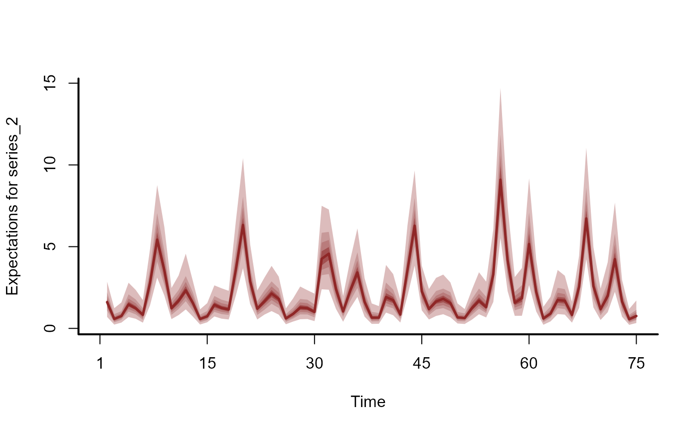
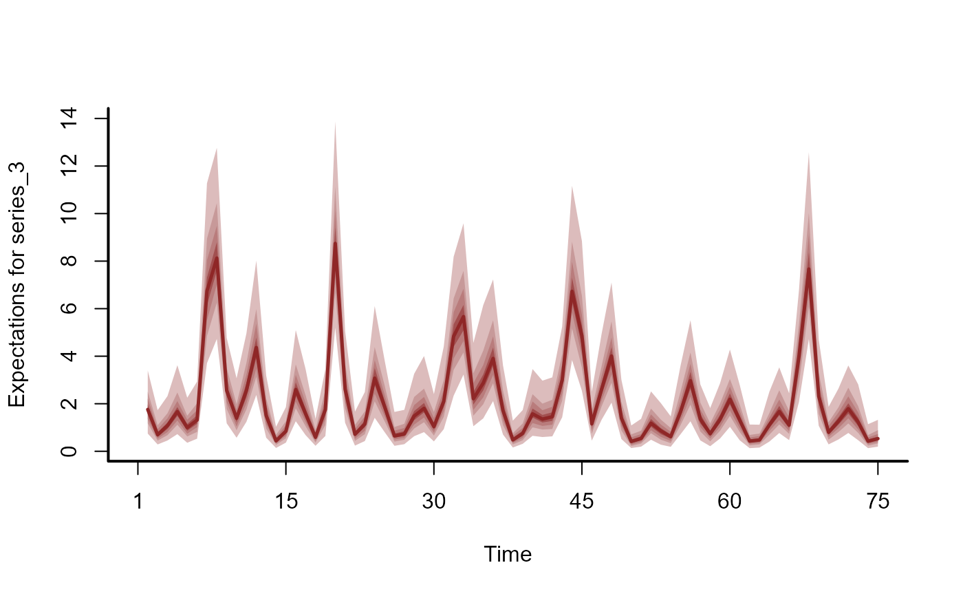
 # Hindcasts as expectations
hc <- hindcast(mod, type = 'expected')
head(summary(hc), 12)
#> # A tibble: 12 × 6
#> series time predQ50 predQ2.5 predQ97.5 type
#> <fct> <int> <dbl> <dbl> <dbl> <chr>
#> 1 series_1 1 0.965 0.475 2.01 expected
#> 2 series_1 2 0.634 0.303 1.50 expected
#> 3 series_1 3 0.447 0.183 0.899 expected
#> 4 series_1 4 0.529 0.216 1.10 expected
#> 5 series_1 5 1.15 0.540 2.28 expected
#> 6 series_1 6 2.83 1.52 5.15 expected
#> 7 series_1 7 4.36 2.47 7.55 expected
#> 8 series_1 8 3.57 2.06 6.80 expected
#> 9 series_1 9 3.24 1.71 5.79 expected
#> 10 series_1 10 2.95 1.38 4.91 expected
#> 11 series_1 11 2.42 1.23 4.20 expected
#> 12 series_1 12 1.07 0.538 2.29 expected
plot(hc, series = 1)
# Hindcasts as expectations
hc <- hindcast(mod, type = 'expected')
head(summary(hc), 12)
#> # A tibble: 12 × 6
#> series time predQ50 predQ2.5 predQ97.5 type
#> <fct> <int> <dbl> <dbl> <dbl> <chr>
#> 1 series_1 1 0.965 0.475 2.01 expected
#> 2 series_1 2 0.634 0.303 1.50 expected
#> 3 series_1 3 0.447 0.183 0.899 expected
#> 4 series_1 4 0.529 0.216 1.10 expected
#> 5 series_1 5 1.15 0.540 2.28 expected
#> 6 series_1 6 2.83 1.52 5.15 expected
#> 7 series_1 7 4.36 2.47 7.55 expected
#> 8 series_1 8 3.57 2.06 6.80 expected
#> 9 series_1 9 3.24 1.71 5.79 expected
#> 10 series_1 10 2.95 1.38 4.91 expected
#> 11 series_1 11 2.42 1.23 4.20 expected
#> 12 series_1 12 1.07 0.538 2.29 expected
plot(hc, series = 1)
 plot(hc, series = 2)
 plot(hc, series = 3)
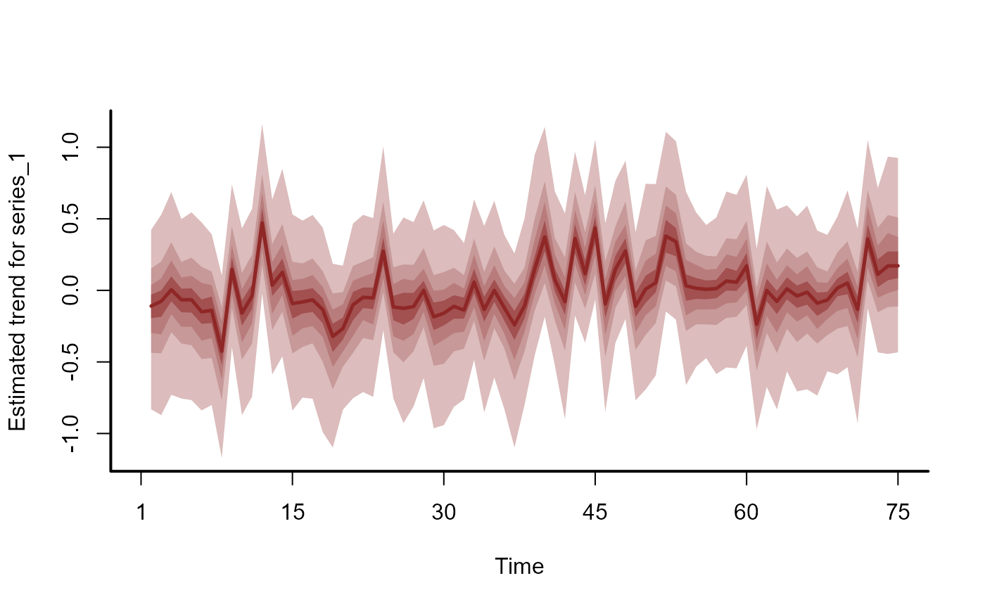
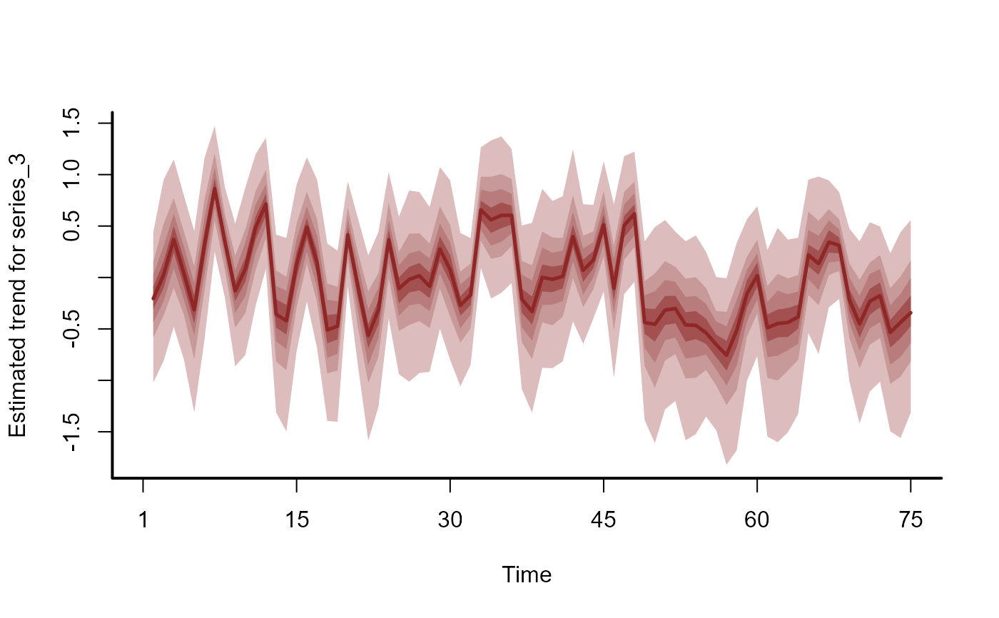
 # Estimated latent trends
hc <- hindcast(mod, type = 'trend')
head(summary(hc), 12)
#> # A tibble: 12 × 6
#> series time predQ50 predQ2.5 predQ97.5 type
#> <fct> <int> <dbl> <dbl> <dbl> <chr>
#> 1 series_1 1 0.0582 -0.520 0.790 trend
#> 2 series_1 2 0.121 -0.466 1.03 trend
#> 3 series_1 3 -0.0438 -0.777 0.614 trend
#> 4 series_1 4 -0.0386 -0.786 0.660 trend
#> 5 series_1 5 0.0565 -0.550 0.680 trend
#> 6 series_1 6 0.0861 -0.465 0.736 trend
#> 7 series_1 7 0.123 -0.372 0.759 trend
#> 8 series_1 8 0.187 -0.304 0.832 trend
#> 9 series_1 9 0.0582 -0.498 0.616 trend
#> 10 series_1 10 -0.182 -0.925 0.275 trend
#> 11 series_1 11 0.0388 -0.552 0.624 trend
#> 12 series_1 12 0.141 -0.456 0.949 trend
plot(hc, series = 1)
# Estimated latent trends
hc <- hindcast(mod, type = 'trend')
head(summary(hc), 12)
#> # A tibble: 12 × 6
#> series time predQ50 predQ2.5 predQ97.5 type
#> <fct> <int> <dbl> <dbl> <dbl> <chr>
#> 1 series_1 1 0.0582 -0.520 0.790 trend
#> 2 series_1 2 0.121 -0.466 1.03 trend
#> 3 series_1 3 -0.0438 -0.777 0.614 trend
#> 4 series_1 4 -0.0386 -0.786 0.660 trend
#> 5 series_1 5 0.0565 -0.550 0.680 trend
#> 6 series_1 6 0.0861 -0.465 0.736 trend
#> 7 series_1 7 0.123 -0.372 0.759 trend
#> 8 series_1 8 0.187 -0.304 0.832 trend
#> 9 series_1 9 0.0582 -0.498 0.616 trend
#> 10 series_1 10 -0.182 -0.925 0.275 trend
#> 11 series_1 11 0.0388 -0.552 0.624 trend
#> 12 series_1 12 0.141 -0.456 0.949 trend
plot(hc, series = 1)
 plot(hc, series = 2)
 plot(hc, series = 3)
 # }
# }