Residual diagnostics for a fitted mvgam object — plot_mvgam

This function takes a fitted mvgam object and returns various residual diagnostic plots

Usage

plot_mvgam_resids(object, series = 1, n_draws = 100L, n_points = 1000L)

Arguments

object: list object returned from mvgam. See mvgam()
series: integer specifying which series in the set is to be plotted
n_draws: integer specifying the number of posterior residual draws to use for calculating uncertainty in the "ACF" and "pACF" frames. Default is 100
n_points: integer specifying the maximum number of points to show in the "Resids vs Fitted" and "Normal Q-Q Plot" frames. Default is 1000

Value

A facetted ggplot object

Details

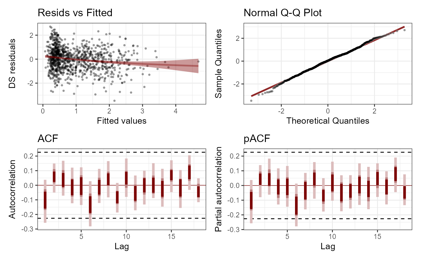
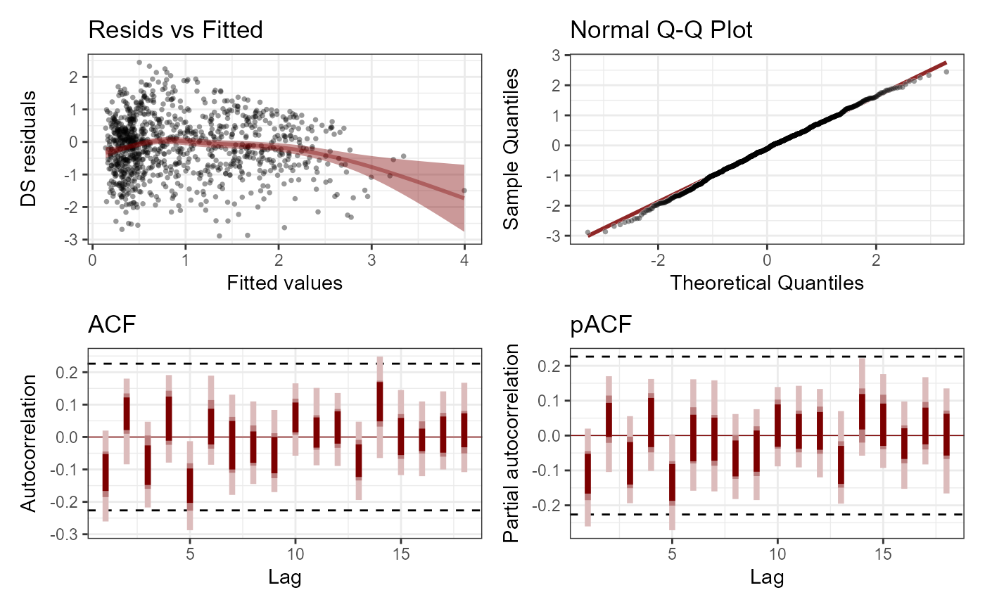
A total of four ggplot plots are generated to examine posterior Dunn-Smyth residuals for the specified series. Plots include a residuals vs fitted values plot, a Q-Q plot, and two plots to check for any remaining temporal autocorrelation in the residuals. Note, all plots only report statistics from a sample of up to 100 posterior draws (to save computational time), so uncertainty in these relationships may not be adequately represented.

Author

Nicholas J Clark

Nicholas J Clark and Matthijs Hollanders

Examples

# \donttest{
simdat <- sim_mvgam(
  n_series = 3,
  trend_model = AR()
)

mod <- mvgam(
  y ~ s(season, bs = 'cc', k = 6),
  trend_model = AR(),
  noncentred = TRUE,
  data = simdat$data_train,
  chains = 2,
  silent = 2
)

# Plot Dunn Smyth residuals for some series
plot_mvgam_resids(mod)

plot_mvgam_resids(mod, series = 2)

# }