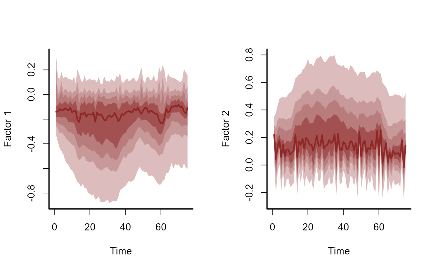
Latent factor summaries for a fitted mvgam object — plot_mvgam

This function takes a fitted mvgam object and returns plots and summary statistics for the latent dynamic factors

Usage

plot_mvgam_factors(object, plot = TRUE)

Arguments

object: list object returned from mvgam. See mvgam()
plot: logical specifying whether factors should be plotted

Value

A dataframe of factor contributions and, optionally, a series of base R plots

Details

If the model in object was estimated using dynamic factors, it is possible that not all factors contributed to the estimated trends. This is due to the regularisation penalty that acts independently on each factor's Gaussian precision, which will squeeze un-needed factors to a white noise process (effectively dropping that factor from the model). In this function, each factor is tested against a null hypothesis of white noise by calculating the sum of the factor's 2nd derivatives. A factor that has a larger contribution will have a larger sum due to the weaker penalty on the factor's precision. If plot == TRUE, the factors are also plotted.

Author

Nicholas J Clark

Examples

# \donttest{
simdat <- sim_mvgam()
mod <- mvgam(y ~ s(season, bs = 'cc',
                  k = 6),
            trend_model = AR(),
            use_lv = TRUE,
            n_lv = 2,
            data = simdat$data_train,
            chains = 2)
#> Warning in 'C:/Users/Nick/AppData/Local/Temp/RtmpCK0CUo/model_0f5e123adc47a9208b1c8eaa9e58906b.stan', line 23, column 31: Found

#>     int division:

#>       n_lv * (n_lv - 1) / 2

#>     Values will be rounded towards zero. If rounding is not desired you can

#>     write

#>     the division as

#>       n_lv * (n_lv - 1) / 2.0

#>     If rounding is intended please use the integer division operator %/%.

#> Compiling Stan program using cmdstanr
#> 
#> Warning in 'C:/Users/Nick/AppData/Local/Temp/RtmpCK0CUo/model-36643e6d335d.stan', line 23, column 33: Found

#>     int division:

#>       n_lv * (n_lv - 1) / 2

#>     Values will be rounded towards zero. If rounding is not desired you can

#>     write

#>     the division as

#>       n_lv * (n_lv - 1) / 2.0

#>     If rounding is intended please use the integer division operator %/%.

#> Start sampling
#> Running MCMC with 2 parallel chains...
#> 
#> Chain 1 Iteration:   1 / 1000 [  0%]  (Warmup) 
#> Chain 2 Iteration:   1 / 1000 [  0%]  (Warmup) 
#> Chain 1 Iteration: 100 / 1000 [ 10%]  (Warmup) 
#> Chain 2 Iteration: 100 / 1000 [ 10%]  (Warmup) 
#> Chain 1 Iteration: 200 / 1000 [ 20%]  (Warmup) 
#> Chain 2 Iteration: 200 / 1000 [ 20%]  (Warmup) 
#> Chain 1 Iteration: 300 / 1000 [ 30%]  (Warmup) 
#> Chain 2 Iteration: 300 / 1000 [ 30%]  (Warmup) 
#> Chain 1 Iteration: 400 / 1000 [ 40%]  (Warmup) 
#> Chain 2 Iteration: 400 / 1000 [ 40%]  (Warmup) 
#> Chain 1 Iteration: 500 / 1000 [ 50%]  (Warmup) 
#> Chain 1 Iteration: 501 / 1000 [ 50%]  (Sampling) 
#> Chain 2 Iteration: 500 / 1000 [ 50%]  (Warmup) 
#> Chain 1 Iteration: 600 / 1000 [ 60%]  (Sampling) 
#> Chain 2 Iteration: 501 / 1000 [ 50%]  (Sampling) 
#> Chain 2 Iteration: 600 / 1000 [ 60%]  (Sampling) 
#> Chain 1 Iteration: 700 / 1000 [ 70%]  (Sampling) 
#> Chain 2 Iteration: 700 / 1000 [ 70%]  (Sampling) 
#> Chain 1 Iteration: 800 / 1000 [ 80%]  (Sampling) 
#> Chain 2 Iteration: 800 / 1000 [ 80%]  (Sampling) 
#> Chain 1 Iteration: 900 / 1000 [ 90%]  (Sampling) 
#> Chain 2 Iteration: 900 / 1000 [ 90%]  (Sampling) 
#> Chain 1 Iteration: 1000 / 1000 [100%]  (Sampling) 
#> Chain 1 finished in 3.4 seconds.
#> Chain 2 Iteration: 1000 / 1000 [100%]  (Sampling) 
#> Chain 2 finished in 3.5 seconds.
#> 
#> Both chains finished successfully.
#> Mean chain execution time: 3.4 seconds.
#> Total execution time: 3.7 seconds.
#> 
plot_mvgam_factors(mod)

#>         Contribution
#> Factor1    0.2016978
#> Factor2    0.7983022
# }