Enhance post-processing of mvgam models using gratia functionality

These evaluation and plotting functions exist to allow some popular gratia methods to work with mvgam or jsdgam models

Usage

drawDotmvgam(
  object,
  trend_effects = FALSE,
  data = NULL,
  select = NULL,
  parametric = FALSE,
  terms = NULL,
  residuals = FALSE,
  scales = c("free", "fixed"),
  ci_level = 0.95,
  n = 100,
  n_3d = 16,
  n_4d = 4,
  unconditional = FALSE,
  overall_uncertainty = TRUE,
  constant = NULL,
  fun = NULL,
  dist = 0.1,
  rug = TRUE,
  contour = TRUE,
  grouped_by = FALSE,
  ci_alpha = 0.2,
  ci_col = "black",
  smooth_col = "black",
  resid_col = "steelblue3",
  contour_col = "black",
  n_contour = NULL,
  partial_match = FALSE,
  discrete_colour = NULL,
  discrete_fill = NULL,
  continuous_colour = NULL,
  continuous_fill = NULL,
  position = "identity",
  angle = NULL,
  ncol = NULL,
  nrow = NULL,
  guides = "keep",
  widths = NULL,
  heights = NULL,
  crs = NULL,
  default_crs = NULL,
  lims_method = "cross",
  wrap = TRUE,
  envir = environment(formula(object)),
  ...
)

eval_smoothDothilbertDotsmooth(
  smooth,
  model,
  n = 100,
  n_3d = NULL,
  n_4d = NULL,
  data = NULL,
  unconditional = FALSE,
  overall_uncertainty = TRUE,
  dist = NULL,
  ...
)

eval_smoothDotmodDotsmooth(
  smooth,
  model,
  n = 100,
  n_3d = NULL,
  n_4d = NULL,
  data = NULL,
  unconditional = FALSE,
  overall_uncertainty = TRUE,
  dist = NULL,
  ...
)

eval_smoothDotmoiDotsmooth(
  smooth,
  model,
  n = 100,
  n_3d = NULL,
  n_4d = NULL,
  data = NULL,
  unconditional = FALSE,
  overall_uncertainty = TRUE,
  dist = NULL,
  ...
)

Arguments

object

a fitted mvgam, the result of a call to mvgam()

trend_effects

logical specifying whether smooth terms from the trend_formula should be drawn. If FALSE, only terms from the observation formula are drawn. If TRUE, only terms from the trend_formula are drawn

data

a data frame of covariate values at which to evaluate the model's smooth functions

select

character, logical, or numeric; which smooths to plot. If NULL, the default, then all model smooths are drawn. Character select matches the labels for smooths as shown for example in the output from summary(object). Logical select operates as per numeric select in the order that smooths are stored

parametric

logical; plot parametric terms also? Note that select is used for selecting which smooths to plot. The terms argument is used to select which parametric effects are plotted. The default, as with mgcv::plot.gam(), is to not draw parametric effects

terms

character; which model parametric terms should be drawn? The Default of NULL will plot all parametric terms that can be drawn.

residuals

currently ignored for mvgam models

scales

character; should all univariate smooths be plotted with the same y-axis scale? If scales = "free", the default, each univariate smooth has its own y-axis scale. If scales = "fixed", a common y axis scale is used for all univariate smooths.

Currently does not affect the y-axis scale of plots of the parametric terms

ci_level

numeric between 0 and 1; the coverage of credible interval.

n

numeric; the number of points over the range of the covariate at which to evaluate the smooth

n_3d, n_4d

numeric; the number of points over the range of last covariate in a 3D or 4D smooth. The default is NULL which achieves the standard behaviour of using n points over the range of all covariate, resulting in n^d evaluation points, where d is the dimension of the smooth. For d > 2 this can result in very many evaluation points and slow performance. For smooths of d > 4, the value of n_4d will be used for all dimensions > 4, unless this is NULL, in which case the default behaviour (using n for all dimensions) will be observed

unconditional

ignored for mvgam models as all appropriate uncertainties are already included in the posterior estimates

overall_uncertainty

ignored for mvgam models as all appropriate uncertainties are already included in the posterior estimates

constant

numeric; a constant to add to the estimated values of the smooth. constant, if supplied, will be added to the estimated value before the confidence band is computed

fun

function; a function that will be applied to the estimated values and confidence interval before plotting. Can be a function or the name of a function. Function fun will be applied after adding any constant, if provided

dist

numeric; if greater than 0, this is used to determine when a location is too far from data to be plotted when plotting 2-D smooths. The data are scaled into the unit square before deciding what to exclude, and dist is a distance within the unit square. See mgcv::exclude.too.far() for further details

rug

logical; draw a rug plot at the bottom of each plot for 1-D smooths or plot locations of data for higher dimensions.

contour

logical; should contours be draw on the plot using ggplot2::geom_contour()

grouped_by

logical; should factor by smooths be drawn as one panel per level of the factor (FALSE, the default), or should the individual smooths be combined into a single panel containing all levels (TRUE)?

ci_alpha

numeric; alpha transparency for confidence or simultaneous interval

ci_col

colour specification for the confidence/credible intervals band. Affects the fill of the interval

smooth_col

colour specification for the smooth line

resid_col

colour specification for residual points. Ignored

contour_col

colour specification for contour lines

n_contour

numeric; the number of contour bins. Will result in n_contour - 1 contour lines being drawn. See ggplot2::geom_contour()

partial_match

logical; should smooths be selected by partial matches with select? If TRUE, select can only be a single string to match against

discrete_colour

a suitable colour scale to be used when plotting discrete variables

discrete_fill

a suitable fill scale to be used when plotting discrete variables.

continuous_colour

a suitable colour scale to be used when plotting continuous variables

continuous_fill

a suitable fill scale to be used when plotting continuous variables

position

Position adjustment, either as a string, or the result of a call to a position adjustment function

angle

numeric; the angle at which the x axis tick labels are to be drawn passed to the angle argument of ggplot2::guide_axis()

ncol, nrow

numeric; the numbers of rows and columns over which to spread the plots

guides

character; one of "keep" (the default), "collect", or "auto". Passed to patchwork::plot_layout()

widths, heights

The relative widths and heights of each column and row in the grid. Will get repeated to match the dimensions of the grid. If there is more than 1 plot and widths = NULL, the value of widths will be set internally to widths = 1 to accommodate plots of smooths that use a fixed aspect ratio.=

crs

the coordinate reference system (CRS) to use for the plot. All data will be projected into this CRS. See ggplot2::coord_sf() for details

default_crs

the coordinate reference system (CRS) to use for the non-sf layers in the plot. If left at the default NULL, the CRS used is 4326 (WGS84), which is appropriate for spline-on-the-sphere smooths, which are parameterized in terms of latitude and longitude as coordinates. See ggplot2::coord_sf() for more details

lims_method

character; affects how the axis limits are determined. See ggplot2::coord_sf(). Be careful; in testing of some examples, changing this to "orthogonal" for example with the chlorophyll-a example from Simon Wood's GAM book quickly used up all the RAM in my test system and the OS killed R. This could be incorrect usage on my part; right now the grid of points at which SOS smooths are evaluated (if not supplied by the user) can produce invalid coordinates for the corners of tiles as the grid is generated for tile centres without respect to the spacing of those tiles

wrap

logical; wrap plots as a patchwork? If FALSE, a list of ggplot objects is returned, 1 per term plotted

envir

an environment to look up the data within

...

additional arguments passed to other methods

smooth

a smooth object of class "gp.smooth" (returned from a model using either the dynamic() function or the gp() function) or of class "moi.smooth" or "mod.smooth" (returned from a model using the 'moi' or 'mod' basis)

model

a fitted mgcv model of clas gam or bam

Details

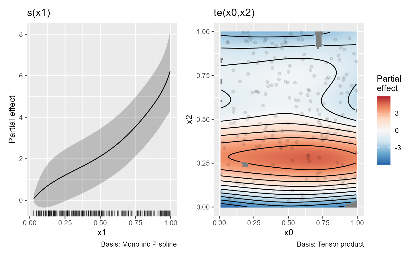
These methods allow mvgam models to be Enhanced if users have the gratia package installed, making available the popular draw() function to plot partial effects of mvgam smooth functions using ggplot2::ggplot() utilities

Author

Nicholas J Clark

Examples

# \donttest{
# Fit a simple GAM and draw partial effects of smooths using 'gratia'
set.seed(0)
dat <- mgcv::gamSim(
  eg = 1,
  n = 200,
  scale = 2
)
#> Gu & Wahba 4 term additive model

mod <- mvgam(
  formula = y ~ s(x1, bs = 'moi') +
    te(x0, x2),
  data = dat,
  family = gaussian(),
  chains = 2,
  silent = 2
)

if (require("gratia")) {
  gratia::draw(mod)
}
#> Loading required package: gratia
#> 
#> Attaching package: ‘gratia’
#> The following object is masked from ‘package:mvgam’:
#> 
#>     add_residuals

# }