Latent variable ordination plots from jsdgam objects

Plot an ordination of latent variables and their factor loadings from jsdgam models

Usage

ordinate(object, ...)

# S3 method for jsdgam
ordinate(
  object,
  which_lvs = c(1, 2),
  biplot = TRUE,
  alpha = 0.5,
  label_sites = TRUE,
  ...
)

Arguments

object

list object of class jsdgam resulting from a call to jsdgam()

...

ignored

which_lvs

A vector of indices indicating the two latent variables to be plotted (if number of the latent variables specified in the model was more than 2). Defaults to c(1, 2)

biplot

Logical. If TRUE, both the site and the species scores will be plotted, with names for the taxa interpreted based on the species argument in the original call to jsdgam(). If FALSE, only the site scores will be plotted

alpha

A proportional numeric scalar between 0 and 1 that controls the relative scaling of the latent variables and their loading coefficients

label_sites

Logical flag. If TRUE, site scores will be plotted as labels using names based on the unit argument in the original call to jsdgam(). If FALSE, site scores will be shown as points only

Value

An ggplot object

Details

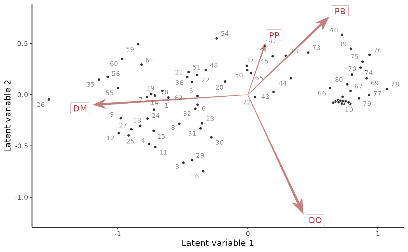
This function constructs a two-dimensional scatterplot in ordination space. The chosen latent variables are first re-rotated using singular value decomposition, so that the first plotted latent variable does not have to be the first latent variable that was estimated in the original model. Posterior median estimates of the variables and the species' loadings on these variables are then used to construct the resulting plot. Some attempt at de-cluttering the resulting plot is made by using geom_label_repel() and geom_text_repel from the ggrepel package, but if there are many sites and/or species then some labels may be removed automatically. Note that you can typically get better, more readable plot layouts if you also have the ggarrow and ggpp packages installed

See also

jsdgam(), residual_cor()

Author

Nicholas J Clark

Examples

# \donttest{
# Fit a JSDGAM to the portal_data captures
mod <- jsdgam(
  formula = captures ~
    # Fixed effects of NDVI and mintemp, row effect as a GP of time
    ndvi_ma12:series + mintemp:series + gp(time, k = 15),
  factor_formula = ~ -1,
  data = portal_data,
  unit = time,
  species = series,
  family = poisson(),
  n_lv = 2,
  silent = 2,
  chains = 2
)

# Plot a residual ordination biplot
ordinate(
  mod,
  alpha = 0.7
)
#> Warning: ggrepel: 17 unlabeled data points (too many overlaps). Consider increasing max.overlaps


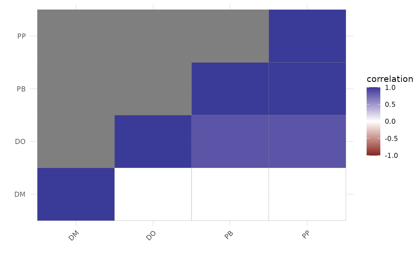
# Compare to a residual correlation plot
plot(
  residual_cor(mod)
)

# }