Compute reactivity, return rates and contributions of interactions to stationary forecast variance from mvgam models with Vector Autoregressive dynamics.
Arguments
- object
listobject of classmvgamresulting from a call tomvgam()that used a Vector Autoregressive latent process model (either asVAR(cor = FALSE)orVAR(cor = TRUE))- ...
Ignored
Details
These measures of stability can be used to assess how important inter-series dependencies are to the variability of a multivariate system and to ask how systems are expected to respond to environmental perturbations. Using the formula for a latent VAR(1) as:
$$ \mu_t \sim \text{MVNormal}(A(\mu_{t - 1}), \Sigma) $$
this function will calculate the long-term stationary forecast distribution of the system, which has mean \(\mu_{\infty}\) and variance \(\Sigma_{\infty}\), to then calculate the following quantities:
prop_int: Proportion of the volume of the stationary forecast distribution that is attributable to lagged interactions: $$ det(A)^2 $$\item `prop_int_adj`: Same as `prop_int` but scaled by the number of series \eqn{p}: \deqn{ det(A)^{2/p} } \item `prop_int_offdiag`: Sensitivity of `prop_int` to inter-series interactions (off-diagonals of \eqn{A}): \deqn{ [2~det(A) (A^{-1})^T] } \item `prop_int_diag`: Sensitivity of `prop_int` to intra-series interactions (diagonals of \eqn{A}): \deqn{ [2~det(A) (A^{-1})^T] } \item `prop_cov_offdiag`: Sensitivity of \eqn{\Sigma_{\infty}} to inter-series error correlations: \deqn{ [2~det(\Sigma_{\infty}) (\Sigma_{\infty}^{-1})^T] } \item `prop_cov_diag`: Sensitivity of \eqn{\Sigma_{\infty}} to error variances: \deqn{ [2~det(\Sigma_{\infty}) (\Sigma_{\infty}^{-1})^T] } \item `reactivity`: Degree to which the system moves away from a stable equilibrium following a perturbation. If \eqn{\sigma_{max}(A)} is the largest singular value of \eqn{A}: \deqn{ \log\sigma_{max}(A) } \item `mean_return_rate`: Asymptotic return rate of the mean of the transition distribution to the stationary mean: \deqn{ \max(\lambda_{A}) } \item `var_return_rate`: Asymptotic return rate of the variance of the transition distribution to the stationary variance: \deqn{ \max(\lambda_{A \otimes A}) }
Major advantages of using mvgam to compute these metrics are that well-calibrated uncertainties are available and that VAR processes are forced to be stationary. These properties make it simple and insightful to calculate and inspect aspects of both long-term and short-term stability.
You can also inspect interactions among the time series in a latent VAR
process using irf for impulse response functions or
fevd for forecast error variance decompositions.
References
AR Ives, B Dennis, KL Cottingham & SR Carpenter (2003). Estimating community stability and ecological interactions from time-series data. Ecological Monographs, 73, 301–330.
Examples
# \dontrun{
# Simulate some time series that follow a latent VAR(1) process
simdat <- sim_mvgam(
family = gaussian(),
n_series = 4,
trend_model = VAR(cor = TRUE),
prop_trend = 1
)
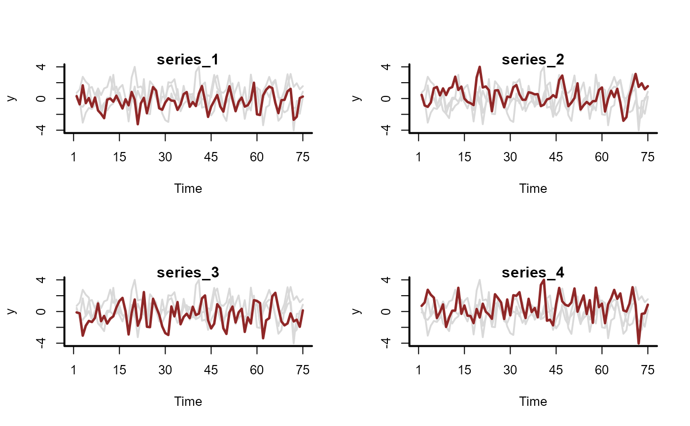
plot_mvgam_series(data = simdat$data_train, series = 'all')
 # Fit a model that uses a latent VAR(1)
mod <- mvgam(
y ~ -1,
trend_formula = ~ 1,
trend_model = VAR(cor = TRUE),
family = gaussian(),
data = simdat$data_train,
chains = 2,
silent = 2
)
# Calculate stability metrics for this system
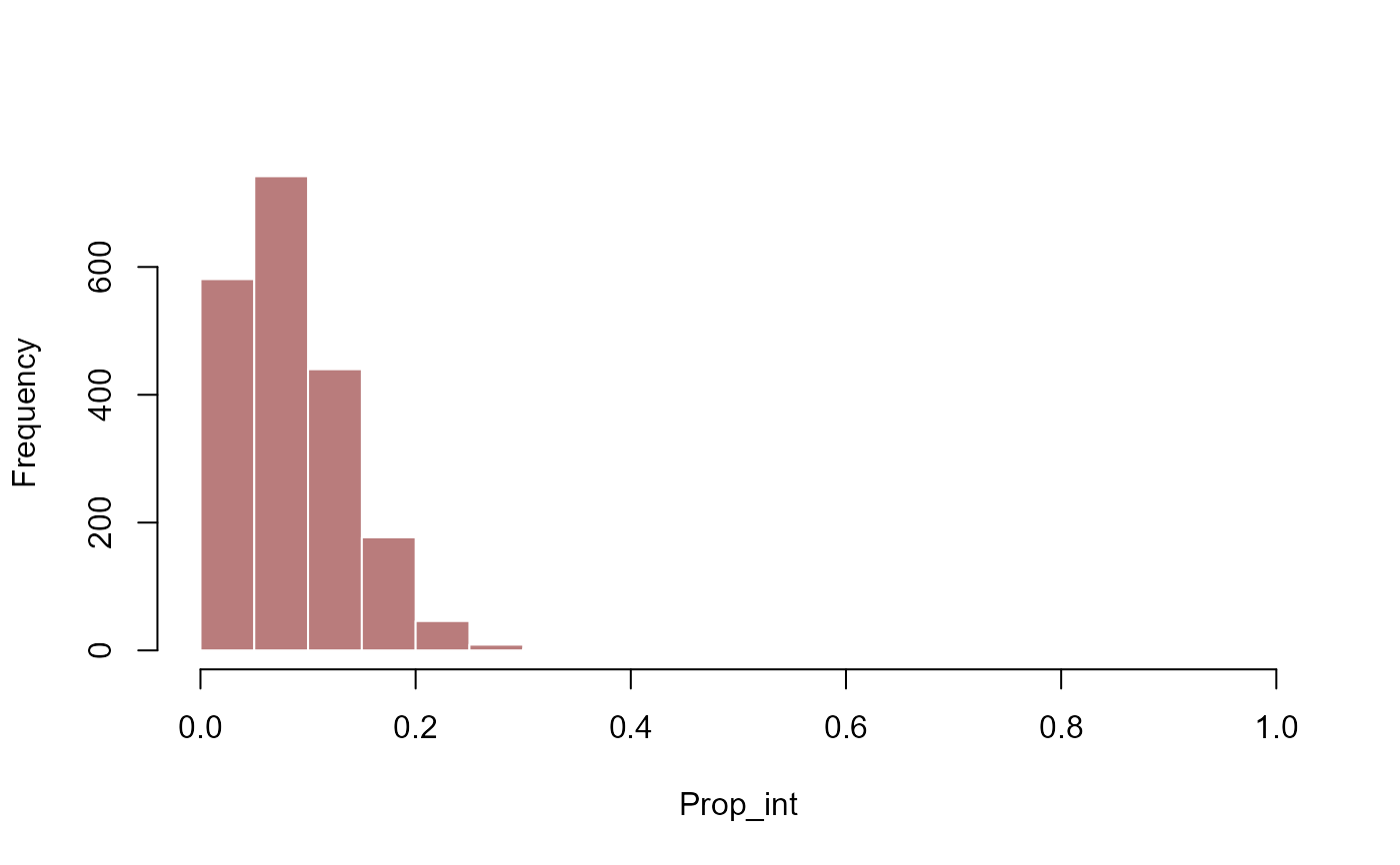
metrics <- stability(mod)
# Proportion of stationary forecast distribution attributable to interactions
hist(
metrics$prop_int,
xlim = c(0, 1),
xlab = 'Prop_int',
main = '',
col = '#B97C7C',
border = 'white'
)
# Fit a model that uses a latent VAR(1)
mod <- mvgam(
y ~ -1,
trend_formula = ~ 1,
trend_model = VAR(cor = TRUE),
family = gaussian(),
data = simdat$data_train,
chains = 2,
silent = 2
)
# Calculate stability metrics for this system
metrics <- stability(mod)
# Proportion of stationary forecast distribution attributable to interactions
hist(
metrics$prop_int,
xlim = c(0, 1),
xlab = 'Prop_int',
main = '',
col = '#B97C7C',
border = 'white'
)
 # Inter- vs intra-series interaction contributions
layout(matrix(1:2, nrow = 2))
hist(
metrics$prop_int_offdiag,
xlim = c(0, 1),
xlab = '',
main = 'Inter-series interactions',
col = '#B97C7C',
border = 'white'
)
hist(
metrics$prop_int_diag,
xlim = c(0, 1),
xlab = 'Contribution to interaction effect',
main = 'Intra-series interactions (density dependence)',
col = 'darkblue',
border = 'white'
)
# Inter- vs intra-series interaction contributions
layout(matrix(1:2, nrow = 2))
hist(
metrics$prop_int_offdiag,
xlim = c(0, 1),
xlab = '',
main = 'Inter-series interactions',
col = '#B97C7C',
border = 'white'
)
hist(
metrics$prop_int_diag,
xlim = c(0, 1),
xlab = 'Contribution to interaction effect',
main = 'Intra-series interactions (density dependence)',
col = 'darkblue',
border = 'white'
)
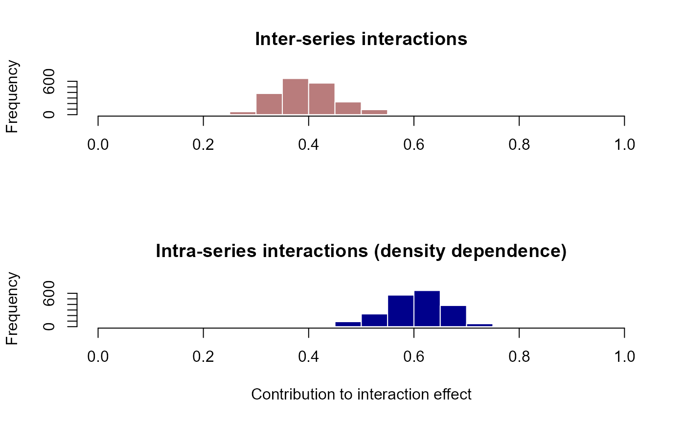 layout(1)
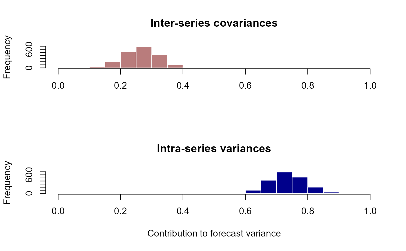
# Inter- vs intra-series contributions to forecast variance
layout(matrix(1:2, nrow = 2))
hist(
metrics$prop_cov_offdiag,
xlim = c(0, 1),
xlab = '',
main = 'Inter-series covariances',
col = '#B97C7C',
border = 'white'
)
hist(
metrics$prop_cov_diag,
xlim = c(0, 1),
xlab = 'Contribution to forecast variance',
main = 'Intra-series variances',
col = 'darkblue',
border = 'white'
)
layout(1)
# Inter- vs intra-series contributions to forecast variance
layout(matrix(1:2, nrow = 2))
hist(
metrics$prop_cov_offdiag,
xlim = c(0, 1),
xlab = '',
main = 'Inter-series covariances',
col = '#B97C7C',
border = 'white'
)
hist(
metrics$prop_cov_diag,
xlim = c(0, 1),
xlab = 'Contribution to forecast variance',
main = 'Intra-series variances',
col = 'darkblue',
border = 'white'
)
 layout(1)
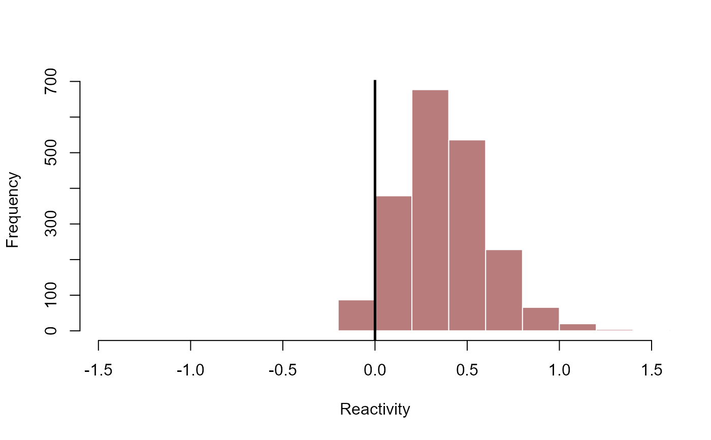
# Reactivity: system response to perturbation
hist(
metrics$reactivity,
main = '',
xlab = 'Reactivity',
col = '#B97C7C',
border = 'white',
xlim = c(
-1 * max(abs(metrics$reactivity)),
max(abs(metrics$reactivity))
)
)
abline(v = 0, lwd = 2.5)
layout(1)
# Reactivity: system response to perturbation
hist(
metrics$reactivity,
main = '',
xlab = 'Reactivity',
col = '#B97C7C',
border = 'white',
xlim = c(
-1 * max(abs(metrics$reactivity)),
max(abs(metrics$reactivity))
)
)
abline(v = 0, lwd = 2.5)
 # }
# }