MultiVariate (Dynamic) Generalized Additive Models
The mvgam 📦 fits Bayesian Dynamic Generalized Additive Models (DGAMs) that can include highly flexible nonlinear predictor effects, latent variables and multivariate time series models. The package does this by relying on functionalities from the impressive brms and mgcv packages. Parameters are estimated using the probabilistic programming language Stan, giving users access to the most advanced Bayesian inference algorithms available. This allows mvgam to fit a very wide range of models, including:
- Multivariate State-Space Time Series Models
- Continuous-Time Autoregressive Time Series Models
- Shared Signal Time Series Models
- Dynamic Factor Models
- Hierarchical N-mixture Models
- Hierarchical Generalized Additive Models
- Joint Species Distribution Models
Installation
Install the stable version from CRAN using: install.packages('mvgam'), or install the development version from GitHub using: devtools::install_github("nicholasjclark/mvgam"). You will also need a working version of Stan installed (along with either rstan and/or cmdstanr). Please refer to installation links for Stan with rstan here, or for Stan with cmdstandr here.

Getting started
mvgam was originally designed to analyse and forecast non-negative integer-valued data (counts). These data are traditionally challenging to analyse with existing time-series analysis packages. But further development of mvgam has resulted in support for a growing number of observation families that extend to other types of data. Currently, the package can handle data for the following families:
-
gaussian()for real-valued data -
student_t()for heavy-tailed real-valued data -
lognormal()for non-negative real-valued data -
Gamma()for non-negative real-valued data -
betar()for proportional data on(0,1) -
bernoulli()for binary data -
poisson()for count data -
nb()for overdispersed count data -
binomial()for count data with known number of trials -
beta_binomial()for overdispersed count data with known number of trials -
nmix()for count data with imperfect detection (unknown number of trials)
See ?mvgam_families for more information. Below is a simple example for simulating and modelling proportional data with Beta observations over a set of seasonal series with independent Gaussian Process dynamic trends:
set.seed(100)
data <- sim_mvgam(
  family = betar(),
  T = 80,
  trend_model = GP(),
  prop_trend = 0.5,
  seasonality = 'shared'
)
Plot the series to see how they evolve over time
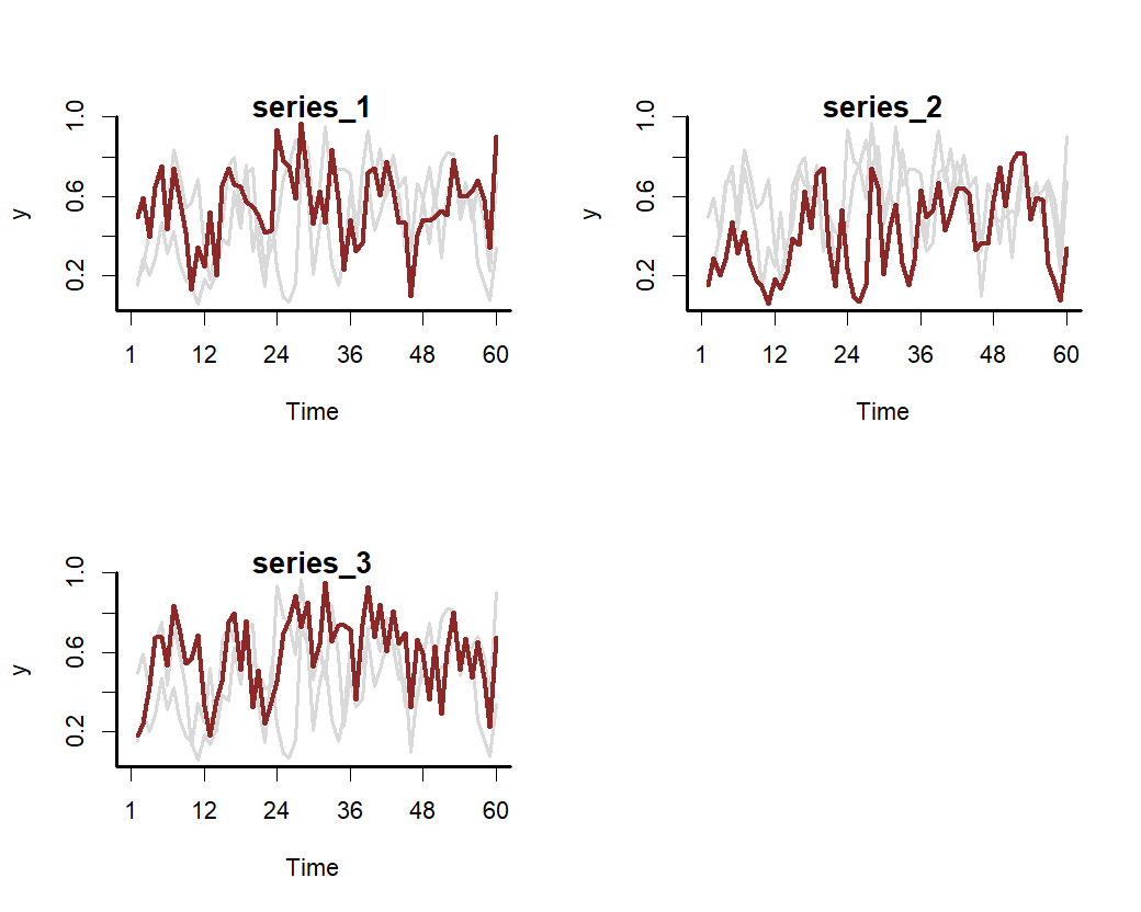
Fit a State-Space GAM to these series that uses a hierarchical cyclic seasonal smooth term to capture variation in seasonality among series. The model also includes series-specific latent Gaussian Processes with squared exponential covariance functions to capture temporal dynamics
mod <- mvgam(
y ~ s(season, bs = 'cc', k = 7) +
s(season, by = series, m = 1, k = 5),
trend_model = GP(),
data = data$data_train,
newdata = data$data_test,
family = betar()
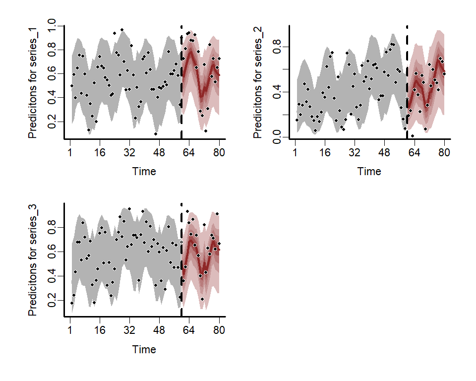
)Plot the estimated posterior hindcast and forecast distributions for each series
library(patchwork)
fc <- forecast(mod)
wrap_plots(
  plot(fc, series = 1),
  plot(fc, series = 2),
  plot(fc, series = 3),
  ncol = 2
)
Various S3 functions can be used to inspect parameter estimates, plot smooth functions and residuals, and evaluate models through posterior predictive checks or forecast comparisons. Please see the package documentation for more detailed examples.
Vignettes
You can set build_vignettes = TRUE when installing but be aware this will slow down the installation drastically. Instead, you can always access the vignette htmls online at https://nicholasjclark.github.io/mvgam/articles/
Citing mvgam and related software
When using any software please make sure to appropriately acknowledge the hard work that developers and maintainers put into making these packages available. Citations are currently the best way to formally acknowledge this work (but feel free to ⭐ the repo as well), so we highly encourage you to cite any packages that you rely on for your research.
When using mvgam, please cite the following:
Clark, N.J. and Wells, K. (2023). Dynamic Generalized Additive Models (DGAMs) for forecasting discrete ecological time series. Methods in Ecology and Evolution. DOI: https://doi.org/10.1111/2041-210X.13974
As mvgam acts as an interface to Stan, please additionally cite:
Carpenter B., Gelman A., Hoffman M. D., Lee D., Goodrich B., Betancourt M., Brubaker M., Guo J., Li P., and Riddell A. (2017). Stan: A probabilistic programming language. Journal of Statistical Software. 76(1). DOI: https://doi.org/10.18637/jss.v076.i01
mvgam relies on several other R packages and, of course, on R itself. Use how_to_cite() after you have fitted a model to simplify the process of finding appropriate citations for your software setup.
Other resources
A number of case studies and step-by-step webinars have been compiled to highlight how GAMs and DGAMs can be useful for analysing multivariate data:
- Time series in R and Stan using the
mvgampackage - Ecological Forecasting with Dynamic Generalized Additive Models
- State-Space Vector Autoregressions in
mvgam - How to interpret and report nonlinear effects from Generalized Additive Models
- Phylogenetic smoothing using mgcv
- Distributed lags (and hierarchical distributed lags) using mgcv and mvgam
- Incorporating time-varying seasonality in forecast models
Getting help
If you encounter a clear bug, please file an issue with a minimal reproducible example on GitHub. Please also feel free to use the mvgam Discussion Board to hunt for or post other discussion topics related to the package, and do check out the mvgam changelog for any updates about recent upgrades that the package has incorporated.
Interested in contributing?
I’m actively seeking PhD students and other researchers to work in the areas of ecological forecasting, multivariate model evaluation and development of mvgam. Please reach out if you are interested (n.clark’at’uq.edu.au). Other contributions are also very welcome, but please see The Contributor Instructions for general guidelines. Note that by participating in this project you agree to abide by the terms of its Contributor Code of Conduct.