Plot conditional posterior predictive checks from mvgam models

Usage

ppc(object, ...)

# S3 method for mvgam
ppc(
  object,
  newdata,
  data_test,
  series = 1,
  type = "hist",
  n_bins,
  legend_position,
  xlab,
  ylab,
  ...
)

Arguments

object: list object returned from mvgam. See mvgam()
...: Further par graphical parameters
newdata: Optional dataframe or list of test data containing at least 'series' and 'time' for the forecast horizon, in addition to any other variables included in the linear predictor of formula. If included, the observed values in the test data are compared to the model's forecast distribution for exploring biases in model predictions. Note this is only useful if the same newdata was also included when fitting the original model.
data_test: Deprecated. Still works in place of newdata but users are recommended to use newdata instead for more seamless integration into R workflows
series: integer specifying which series in the set is to be plotted
type: character specifying the type of posterior predictive check to calculate and plot. Valid options are: 'rootogram', 'mean', 'hist', 'density', 'prop_zero', 'pit' and 'cdf'
n_bins: integer specifying the number of bins to use for binning observed values when plotting a rootogram or histogram. Default is 50 bins for a rootogram, which means that if there are >50 unique observed values, bins will be used to prevent overplotting and facilitate interpretation. Default for a histogram is to use the number of bins returned by a call to hist in base R
legend_position: The location may also be specified by setting x to a single keyword from the list "bottomright", "bottom", "bottomleft", "left", "topleft", "top", "topright", "right" and "center". This places the legend on the inside of the plot frame at the given location. Or alternatively, use "none" to hide the legend.
xlab: Label for x axis
ylab: Label for y axis

Value

A base R graphics plot showing either a posterior rootogram (for type == 'rootogram'), the predicted vs observed mean for the series (for type == 'mean'), predicted vs observed proportion of zeroes for the series (for type == 'prop_zero'), predicted vs observed histogram for the series (for type == 'hist'), kernel density or empirical CDF estimates for posterior predictions (for type == 'density' or type == 'cdf') or a Probability Integral Transform histogram (for type == 'pit').

Details

Conditional posterior predictions are drawn from the fitted mvgam and compared against the empirical distribution of the observed data for a specified series to help evaluate the model's ability to generate unbiased predictions. For all plots apart from type = 'rootogram', posterior predictions can also be compared to out of sample observations as long as these observations were included as 'data_test' in the original model fit and supplied here. Rootograms are currently only plotted using the 'hanging' style.

Note that the predictions used for these plots are conditional on the observed data, i.e. they are those predictions that have been generated directly within the mvgam() model. They can be misleading if the model included flexible dynamic trend components. For a broader range of posterior checks that are created using unconditional "new data" predictions, see pp_check.mvgam

Author

Nicholas J Clark

Examples

# \donttest{
# Simulate some smooth effects and fit a model
set.seed(0)

dat <- mgcv::gamSim(
  1,
  n = 200,
  scale = 2
)
#> Gu & Wahba 4 term additive model

mod <- mvgam(
  y ~ s(x0) + s(x1) + s(x2) + s(x3),
  data = dat,
  family = gaussian(),
  chains = 2,
  silent = 2
)

# Posterior checks
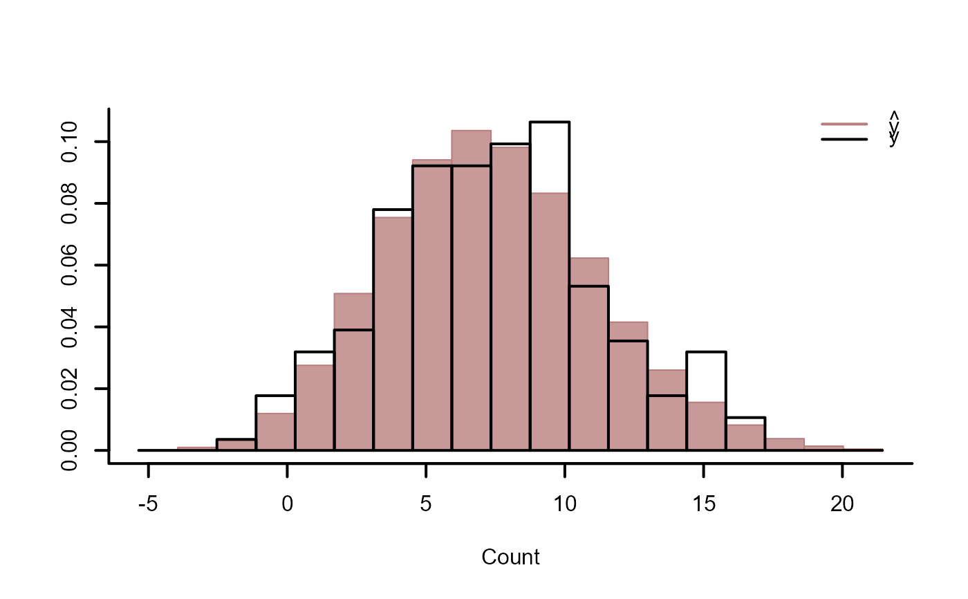
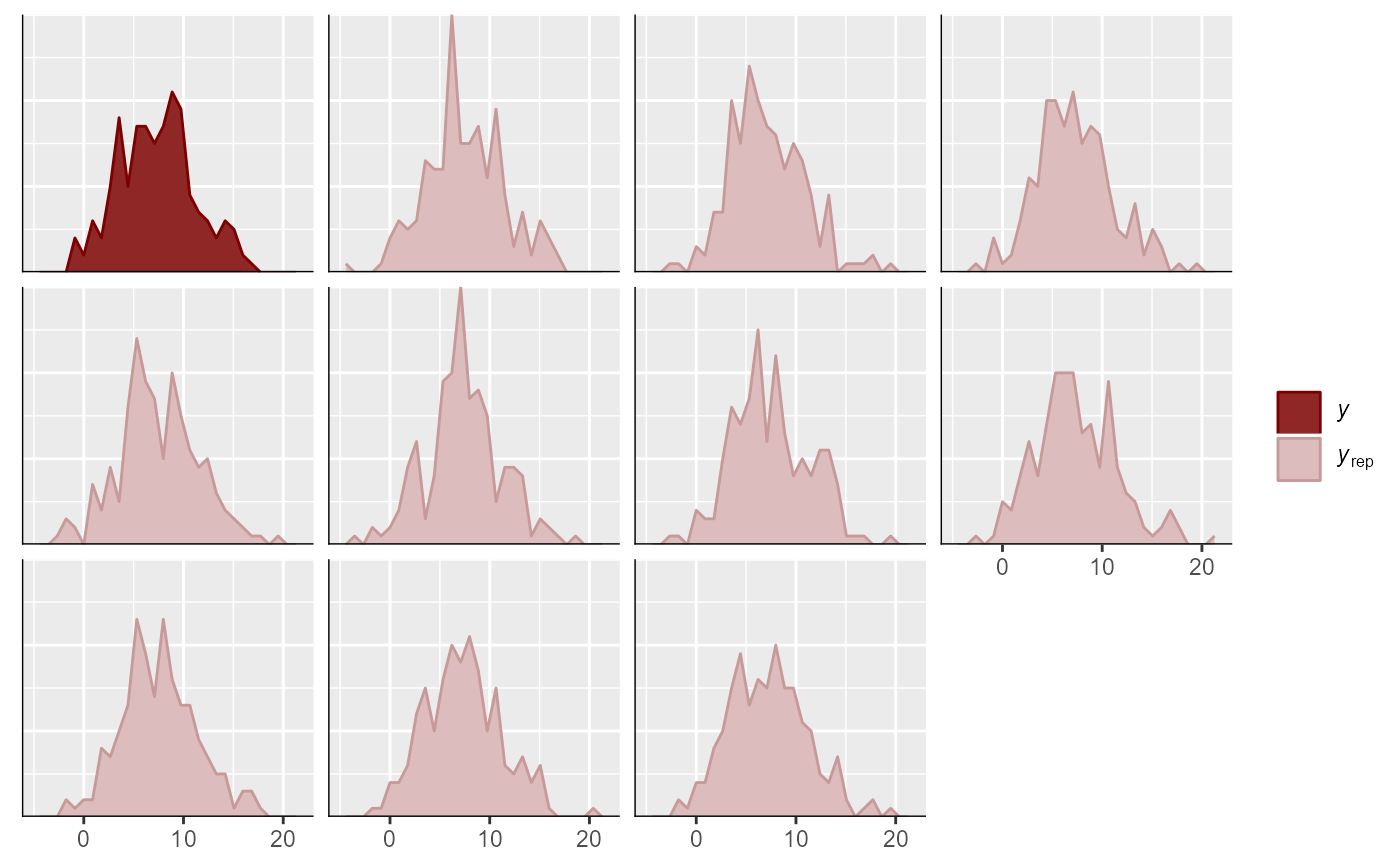
ppc(mod, type = "hist")

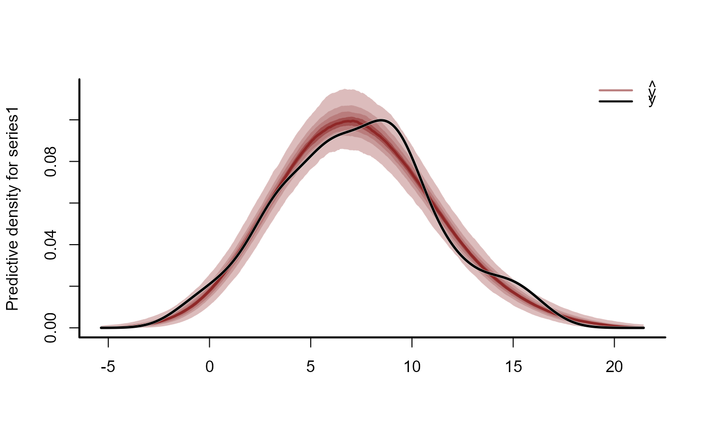
ppc(mod, type = "density")

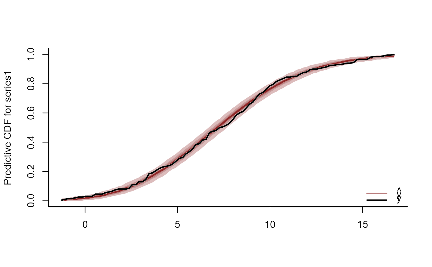
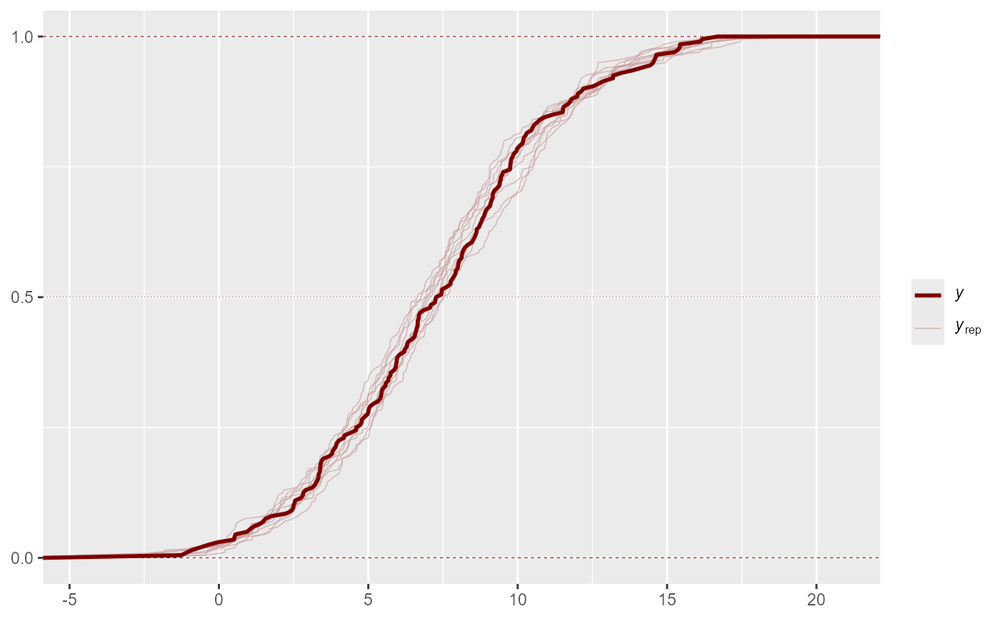
ppc(mod, type = "cdf")


# Many more options are available with pp_check()
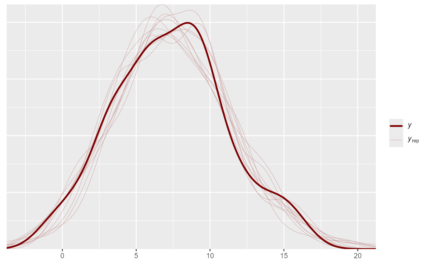
pp_check(mod)
#> Using 10 posterior draws for ppc type 'dens_overlay' by default.

pp_check(mod, type = "ecdf_overlay")
#> Using 10 posterior draws for ppc type 'ecdf_overlay' by default.

pp_check(mod, type = "freqpoly")
#> Using 10 posterior draws for ppc type 'freqpoly' by default.
#> `stat_bin()` using `bins = 30`. Pick better value with `binwidth`.

# }