ffc

Functional ForeCasting

The goal of the ffc 📦 is to forecast complex, time-changing functional relationships by integrating Generalized Additive Models with dynamic factor functional basis expansions.

Key benefits:

Model functional responses that change shape over time (not just magnitude)
Forecast entire curves into the future, not just single values
Handle complex multivariate time series with functional structure
Seamless integration with the powerful mgcv and fable ecosystems

The package introduces dynamic functional predictors using the new fts() term, which decomposes functional time series into time-varying basis coefficients that can be forecasted using either independent time series models from the fable package or with efficient dynamic factor models using precompiled Stan models.

Installation

You can install the development version of ffc from GitHub with:

# install.packages("pak")
pak::pak("nicholasjclark/ffc")

Quick Start

library(ffc)

# Fit a model with time-varying coefficients
mod <- ffc_gam(
  response ~ fts(predictor, time_k = 10),  
  data = your_data,
  time = "time_column",
  family = gaussian()
)

# Forecast the functional coefficients
fc <- forecast(mod, newdata = future_data, model = "ARDF")

Examples

Tourism Forecasting with `fabletools` Integration

library(fable)
library(tsibble)
library(tidyverse)
library(ggplot2); theme_set(theme_bw(base_size = 12))

Our aim here is to forecast the number of domestic visitors to Melbourne, Australia. The data can be found in the tsibble::tourism data set. For now we need to explicitly add the quarter and time variables to the data, but in future this will be done automatically for seamless integration with the tsibbleverse

tourism_melb <- tourism |>
  filter(
    Region == "Melbourne",
    Purpose == "Visiting"
  ) |>
  mutate(
    quarter = lubridate::quarter(Quarter),
    time = dplyr::row_number()
  )
tourism_melb
#> # A tsibble: 80 x 7 [1Q]
#> # Key:       Region, State, Purpose [1]
#>    Quarter Region    State    Purpose  Trips quarter  time
#>      <qtr> <chr>     <chr>    <chr>    <dbl>   <int> <int>
#>  1 1998 Q1 Melbourne Victoria Visiting  666.       1     1
#>  2 1998 Q2 Melbourne Victoria Visiting  601.       2     2
#>  3 1998 Q3 Melbourne Victoria Visiting  529.       3     3
#>  4 1998 Q4 Melbourne Victoria Visiting  575.       4     4
#>  5 1999 Q1 Melbourne Victoria Visiting  623.       1     5
#>  6 1999 Q2 Melbourne Victoria Visiting  530.       2     6
#>  7 1999 Q3 Melbourne Victoria Visiting  479.       3     7
#>  8 1999 Q4 Melbourne Victoria Visiting  538.       4     8
#>  9 2000 Q1 Melbourne Victoria Visiting  618.       1     9
#> 10 2000 Q2 Melbourne Victoria Visiting  549.       2    10
#> # ℹ 70 more rows

Split into training and testing folds. We wil aim to forecast the last 5 quarters of the data

train <- tourism_melb |>
  dplyr::slice_head(n = 75)

test <- tourism_melb |>
  dplyr::slice_tail(n = 5)

Now fit an ffc_gam. We use time-varying level and time-varying seasonality components, together with a Tweedie observation model (because our outcome, Trips, consists of non-negative real values). This model is simpler so we use the 'gam' engine for fitting:

mod <- ffc_gam(
  Trips ~
    # Use mean_only = TRUE to model a time-varying mean
    fts(
      time,
      mean_only = TRUE,
      time_k = 50,
      time_m = 1
    ) +
    # Time-varying seasonality
    fts(
      quarter,
      k = 4,
      time_k = 15,
      time_m = 1
    ),
  time = "time",
  data = train,
  family = tw(),
  engine = "gam"
)

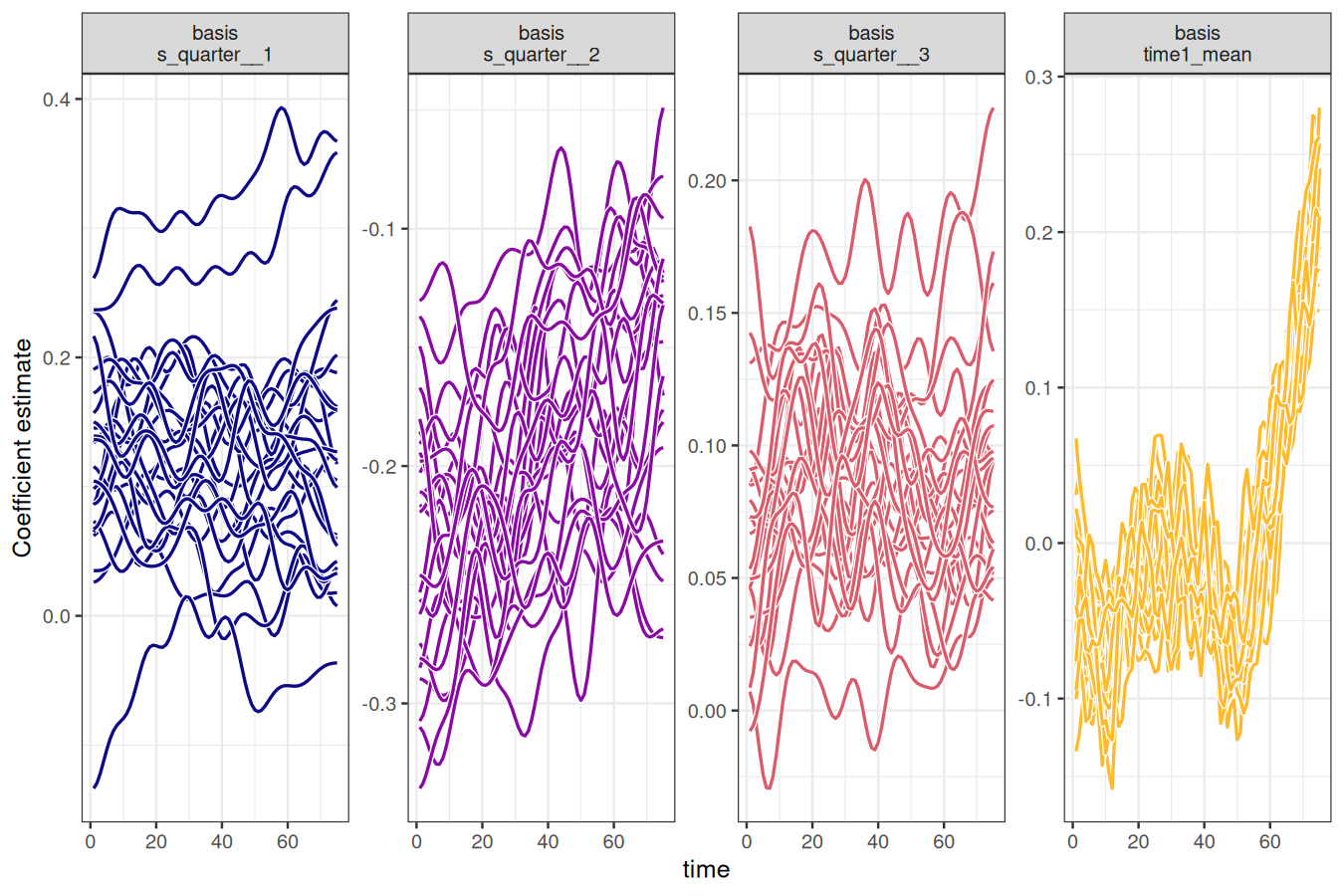
The autoplot() method is handy for viewing the time-varying basis coefficients from ffc_gam() models. Here we draw 10 realisations from the estimated coefficient distributions and plot them.

fts_coefs(mod, times = 10, summary = FALSE) |>
  autoplot()

autplot() plots showing time-varying coefficients for the tourism model, illustrating how basis coefficients have been estimated to vary through time.

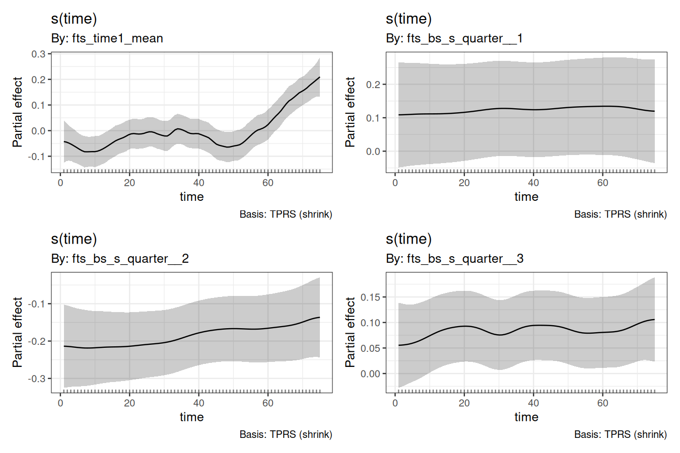
We can also draw the time-varying basis coefficients using support from the gratia package, which has helpful functions for plotting smooth effects:

gratia::draw(mod)

Smooth plots showing time-varying coefficients for the tourism model. The upper panel shows the time-varying level component while the lower panel displays seasonal coefficients that change over time, demonstrating how seasonality patterns evolve.

These plots show the time-varying coefficients for a set of basis functions. We have one function representing the mean of the series (essentially a constant) as well as three basis functions representing the quarterly seasonality. Each of these has a coefficient that can change through time, allowing the entire functional series to change shape over time. We can compute forecast distribution by fitting the basis coefficient forecast models in parallel (which is automatically supported within the fable package). Here we fit independent exponential smoothing models to each coefficient time series

fc <- forecast(
  object = mod,
  newdata = test,
  model = "ETS",
  summary = FALSE
)

We can also convert resulting forecasts to a fable object for automatic plotting and/or scoring of forecasts

# Using the new as_fable method for seamless conversion
fc_ffc <- as_fable(mod, newdata = test, forecasts = fc)
fc_ffc
#> # A fable: 5 x 10 [1Q]
#> # Key:     Region, State, Purpose [1]
#>   Quarter Region    State   Purpose Trips quarter  time       .dist .mean .model
#>     <qtr> <chr>     <chr>   <chr>   <dbl>   <int> <int>      <dist> <dbl> <chr> 
#> 1 2016 Q4 Melbourne Victor… Visiti…  804.       4    76 sample[200]  839. FFC_E…
#> 2 2017 Q1 Melbourne Victor… Visiti…  734.       1    77 sample[200]  760. FFC_E…
#> 3 2017 Q2 Melbourne Victor… Visiti…  670.       2    78 sample[200]  774. FFC_E…
#> 4 2017 Q3 Melbourne Victor… Visiti…  824.       3    79 sample[200]  747. FFC_E…
#> 5 2017 Q4 Melbourne Victor… Visiti…  985.       4    80 sample[200]  836. FFC_E…

Leverage the fabletools ecosystem for forecast analysis

# Calculate accuracy metrics
accuracy(fc_ffc, test)
#> # A tibble: 1 × 13
#>   .model  Region   State Purpose .type    ME  RMSE   MAE   MPE  MAPE  MASE RMSSE
#>   <chr>   <chr>    <chr> <chr>   <chr> <dbl> <dbl> <dbl> <dbl> <dbl> <dbl> <dbl>
#> 1 FFC_ETS Melbour… Vict… Visiti… Test   11.9  90.6  78.4 0.165  9.60   NaN   NaN
#> # ℹ 1 more variable: ACF1 <dbl>

# Generate prediction intervals  
fc_intervals <- hilo(fc_ffc, level = c(80, 95))
fc_intervals
#> # A tsibble: 5 x 12 [1Q]
#> # Key:       Region, State, Purpose [1]
#>   Quarter Region    State   Purpose Trips quarter  time       .dist .mean .model
#>     <qtr> <chr>     <chr>   <chr>   <dbl>   <int> <int>      <dist> <dbl> <chr> 
#> 1 2016 Q4 Melbourne Victor… Visiti…  804.       4    76 sample[200]  839. FFC_E…
#> 2 2017 Q1 Melbourne Victor… Visiti…  734.       1    77 sample[200]  760. FFC_E…
#> 3 2017 Q2 Melbourne Victor… Visiti…  670.       2    78 sample[200]  774. FFC_E…
#> 4 2017 Q3 Melbourne Victor… Visiti…  824.       3    79 sample[200]  747. FFC_E…
#> 5 2017 Q4 Melbourne Victor… Visiti…  985.       4    80 sample[200]  836. FFC_E…
#> # ℹ 2 more variables: `80%` <hilo>, `95%` <hilo>

# Distribution summaries
fc_summary <- fc_ffc |>
  summarise(
    mean_forecast = mean(.dist),
    median_forecast = median(.dist),
    q25 = quantile(.dist, 0.25), 
    q75 = quantile(.dist, 0.75)
  )
fc_summary
#> # A tsibble: 5 x 5 [1Q]
#>   Quarter mean_forecast median_forecast   q25   q75
#>     <qtr>         <dbl>           <dbl> <dbl> <dbl>
#> 1 2016 Q4          839.            843.  778.  896.
#> 2 2017 Q1          760.            758.  711.  815.
#> 3 2017 Q2          774.            770.  730.  822.
#> 4 2017 Q3          747.            743.  695.  802.
#> 5 2017 Q4          836.            831.  785.  898.

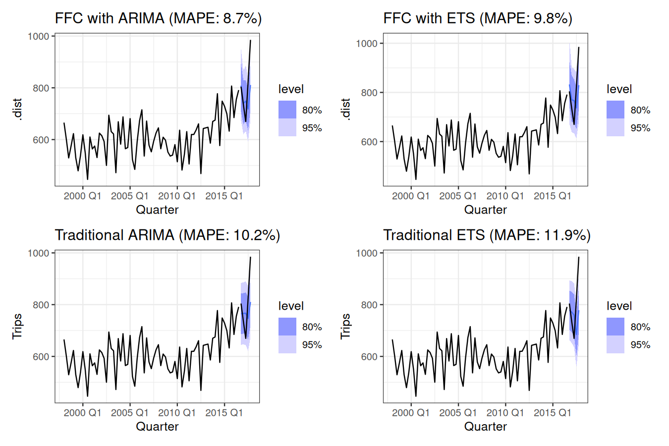
Next we can explore how to compare forecasts from ffc models to traditional time series models by again leveraging the simplicity and power of the fable ecosystem

# Generate FFC forecasts with different models
fc_ffc_arima <- as_fable(mod, newdata = test, model = "ARIMA")
fc_ffc_ets <- as_fable(mod, newdata = test, model = "ETS")

# Generate traditional model forecasts
fc_traditional <- train |>
  model(
    ARIMA = ARIMA(Trips),
    ETS = ETS(Trips)
  ) |>
  forecast(h = 5)

# Calculate accuracy for all models
acc_ffc_arima <- accuracy(fc_ffc_arima, test)
acc_ffc_ets <- accuracy(fc_ffc_ets, test)
acc_traditional <- accuracy(fc_traditional, test)

# Extract MAPE values for titles
mape_ffc_arima <- round(acc_ffc_arima$MAPE, 1)
mape_ffc_ets <- round(acc_ffc_ets$MAPE, 1)
mape_arima <- round(acc_traditional$MAPE[acc_traditional$.model == "ARIMA"], 1)
mape_ets <- round(acc_traditional$MAPE[acc_traditional$.model == "ETS"], 1)

# Create comparison plots
library(patchwork)

p1 <- autoplot(fc_ffc_arima, train) + 
  geom_line(data = test, aes(y = Trips), color = "black") +
  ggtitle(paste0("FFC with ARIMA (MAPE: ", mape_ffc_arima, "%)"))

p2 <- autoplot(fc_ffc_ets, train) + 
  geom_line(data = test, aes(y = Trips), color = "black") +
  ggtitle(paste0("FFC with ETS (MAPE: ", mape_ffc_ets, "%)"))

p3 <- autoplot(filter(fc_traditional, .model == "ARIMA"), train) +
  geom_line(data = test, aes(y = Trips), color = "black") +
  ggtitle(paste0("Traditional ARIMA (MAPE: ", mape_arima, "%)"))

p4 <- autoplot(filter(fc_traditional, .model == "ETS"), train) +
  geom_line(data = test, aes(y = Trips), color = "black") +
  ggtitle(paste0("Traditional ETS (MAPE: ", mape_ets, "%)"))

(p1 | p2) / (p3 | p4)

Comprehensive model comparison showing FFC functional forecasting versus traditional ARIMA and ETS models for Melbourne tourism data. The plot demonstrates forecast performance with MAPE values in titles, revealing the added value of functional forecasting approaches.

These plots illustrate how the ffc models outperform traditional forecasting models for this forecasting experiment by thinking about this as a functional time series problem.

Getting help

If you encounter a clear bug, please file an issue with a minimal reproducible example on GitHub

Contributing

Contributions are very welcome, but please see our Code of Conduct when you are considering changes that you would like to make.

License

The ffc project is licensed under an MIT open source license