Fit a functional time series model using dynamic functional coefficients

Fit Generalized Additive Models that can include time-varying (dynamic) functions

Usage

ffc_gam(
  formula,
  family = gaussian(),
  data = list(),
  time,
  engine = c("gam", "bam"),
  ...
)

Arguments

formula: A GAM formula (see formula.gam and also gam.models). This is exactly like the formula for a GLM except that smooth terms, fts(), s() and te() can be added to the right hand side to specify that the linear predictor depends on smooth functions of predictors (or linear functionals of these).
family: This is a family object specifying the distribution and link to use in fitting etc. See glm and family for more details. The extended families listed in family.mgcv can also be used.
data: A data.frame containing the variables in the model. Unlike gam, ffc_gam requires data to be a data.frame and does not support list data structures.
time: character specifying which variable in data represents the the time ordering of the observations
engine: character string specifying which mgcv interface to use for fitting the model.
...: other arguments to pass to either gam

Value

An object of class ffc_gam, which inherits from objects of class gam or bam. Use methods(class = "ffc_gam") to see available methods.

Details

This function will update the supplied formula to ensure any time-varying functionals (supplied through fts() terms in the formula right hand side) are appropriately incorporated into the model. It then passes the updated model and data objects to the specified engine for model fitting

Author

Nicholas J Clark

Examples

# Fit a dynamic function-on-function regression to the Queensland
# mortality data
data("qld_mortality")
mod <- ffc_gam(
  deaths ~
    offset(log(population)) +
    sex +
    fts(age,
      k = 8,
      time_k = 10
    ),
  time = "year",
  data = qld_mortality,
  family = poisson(),
  engine = "bam"
)
class(mod)
#> [1] "ffc_gam" "bam"     "gam"     "glm"     "lm"     
summary(mod)
#> 
#> Family: poisson 
#> Link function: log 
#> 
#> Formula:
#> deaths ~ sex + offset(log(population)) + s(year, by = fts_bs_s_age__1, 
#>     bs = "ts", k = 10, m = 2, id = 1) + s(year, by = fts_bs_s_age__2, 
#>     bs = "ts", k = 10, m = 2, id = 1) + s(year, by = fts_bs_s_age__3, 
#>     bs = "ts", k = 10, m = 2, id = 1) + s(year, by = fts_bs_s_age__4, 
#>     bs = "ts", k = 10, m = 2, id = 1) + s(year, by = fts_bs_s_age__5, 
#>     bs = "ts", k = 10, m = 2, id = 1) + s(year, by = fts_bs_s_age__6, 
#>     bs = "ts", k = 10, m = 2, id = 1) + s(year, by = fts_bs_s_age__7, 
#>     bs = "ts", k = 10, m = 2, id = 1)
#> 
#> Parametric coefficients:
#>              Estimate Std. Error z value Pr(>|z|)    
#> (Intercept) -5.553606   0.002381 -2332.6   <2e-16 ***
#> sexmale      0.472665   0.002077   227.6   <2e-16 ***
#> ---
#> Signif. codes:  0 ‘***’ 0.001 ‘**’ 0.01 ‘*’ 0.05 ‘.’ 0.1 ‘ ’ 1
#> 
#> Approximate significance of smooth terms:
#>                           edf Ref.df Chi.sq p-value    
#> s(year):fts_bs_s_age__1 8.165     10  22396  <2e-16 ***
#> s(year):fts_bs_s_age__2 6.829     10  15647  <2e-16 ***
#> s(year):fts_bs_s_age__3 8.112     10   2883  <2e-16 ***
#> s(year):fts_bs_s_age__4 7.085     10  14643  <2e-16 ***
#> s(year):fts_bs_s_age__5 7.847     10    707  <2e-16 ***
#> s(year):fts_bs_s_age__6 5.923     10  23037  <2e-16 ***
#> s(year):fts_bs_s_age__7 6.259     10   8424  <2e-16 ***
#> ---
#> Signif. codes:  0 ‘***’ 0.001 ‘**’ 0.01 ‘*’ 0.05 ‘.’ 0.1 ‘ ’ 1
#> 
#> R-sq.(adj) =  0.972   Deviance explained = 94.7%
#> fREML =  46558  Scale est. = 1         n = 8282

# Distributional regression with gaulss() family
# Simulated data with time-varying location and scale
library(mgcv)
#> Loading required package: nlme
#> 
#> Attaching package: ‘nlme’
#> The following object is masked from ‘package:dplyr’:
#> 
#>     collapse
#> This is mgcv 1.9-3. For overview type 'help("mgcv-package")'.
set.seed(1234)
n <- 50
sim_data <- data.frame(
  time = 1:n,
  x = rnorm(n),
  y = rnorm(n, mean = sin(2 * pi * (1:n) / 20),
            sd = 0.5 + 0.3 * cos(2 * pi * (1:n) / 15))
)

# Fit distributional model with time-varying parameters
dist_mod <- ffc_gam(
  list(
    y ~ fts(x, k = 5),      # Location parameter
    ~ fts(x, k = 3)         # Scale parameter
  ),
  family = gaulss(),
  data = sim_data,
  time = "time"
)
#> Warning: Shared penalties may cause fitting issues with distributional families. Setting {.field share_penalty} = FALSE.
#> This warning is displayed once per session.

# Extract parameter-specific coefficients
coefs <- fts_coefs(dist_mod)
print(unique(coefs$.parameter))  # Shows "location" and "scale"
#> [1] "location" "scale"   

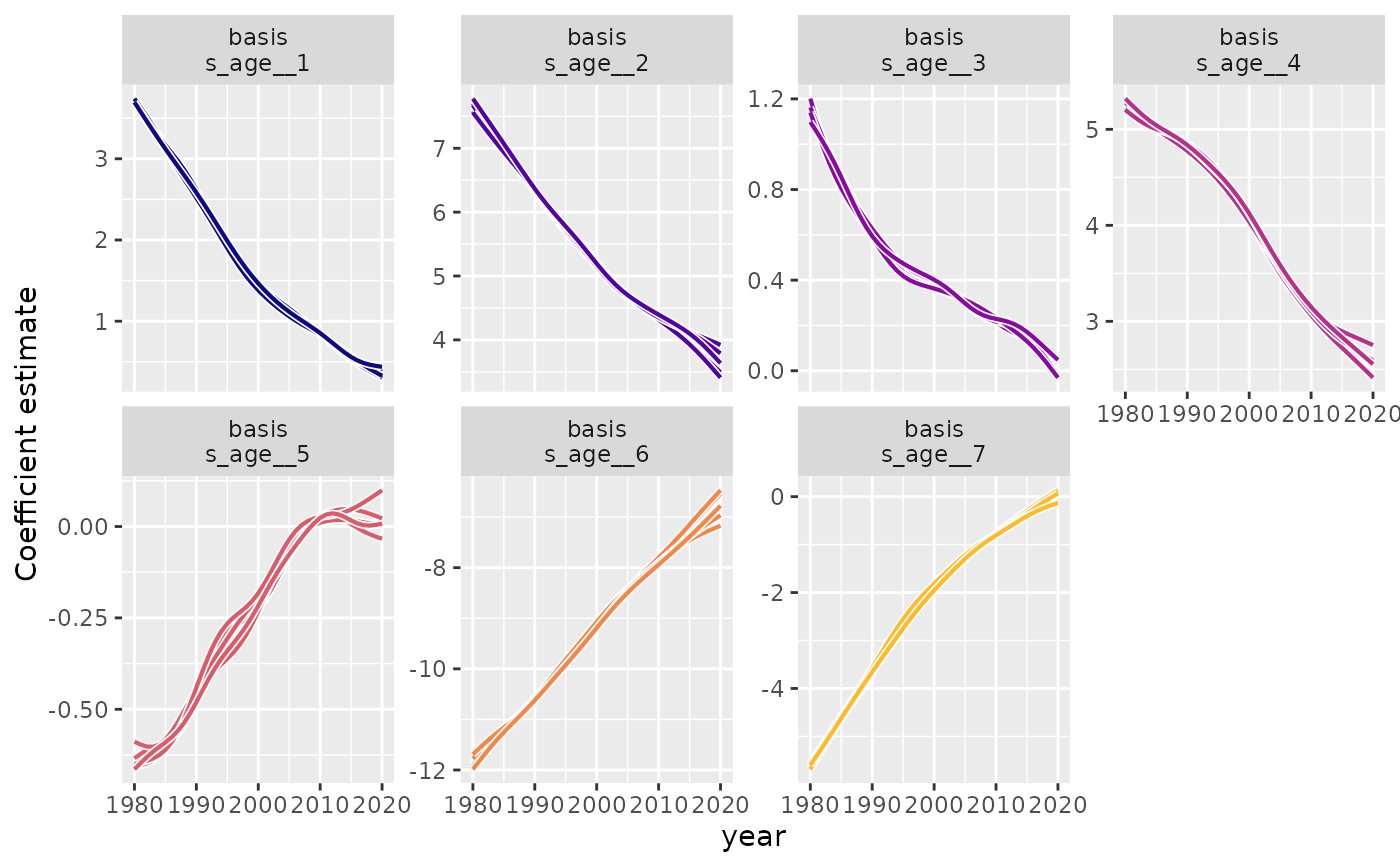
# Extract and visualize time-varying coefficients
coefs <- fts_coefs(mod, summary = FALSE, n_samples = 5)
autoplot(coefs)


# Forecast future mortality patterns
future_data <- expand.grid(
  age = unique(qld_mortality$age),
  sex = unique(qld_mortality$sex),
  year = 2021:2025,
  # Use rate scale (to predict deaths per person)
  population = 1
)

# Generate forecasts using ETS model for coefficients
mortality_fc <- forecast(mod, newdata = future_data, model = "ETS",
                         type = "expected")
head(mortality_fc)
#> # A tibble: 6 × 6
#>   .estimate  .error    .q2.5     .q10     .q90   .q97.5
#>       <dbl>   <dbl>    <dbl>    <dbl>    <dbl>    <dbl>
#> 1  0.00115  0.00119 0.000997 0.00104  0.00130  0.00138 
#> 2  0.00102  0.00132 0.000883 0.000936 0.00115  0.00120 
#> 3  0.000904 0.00147 0.000759 0.000822 0.00105  0.00111 
#> 4  0.000804 0.00152 0.000694 0.000736 0.000913 0.00104 
#> 5  0.000714 0.00160 0.000616 0.000658 0.000823 0.000894
#> 6  0.000638 0.00168 0.000545 0.000578 0.000728 0.000812