Ecological forecasting in R

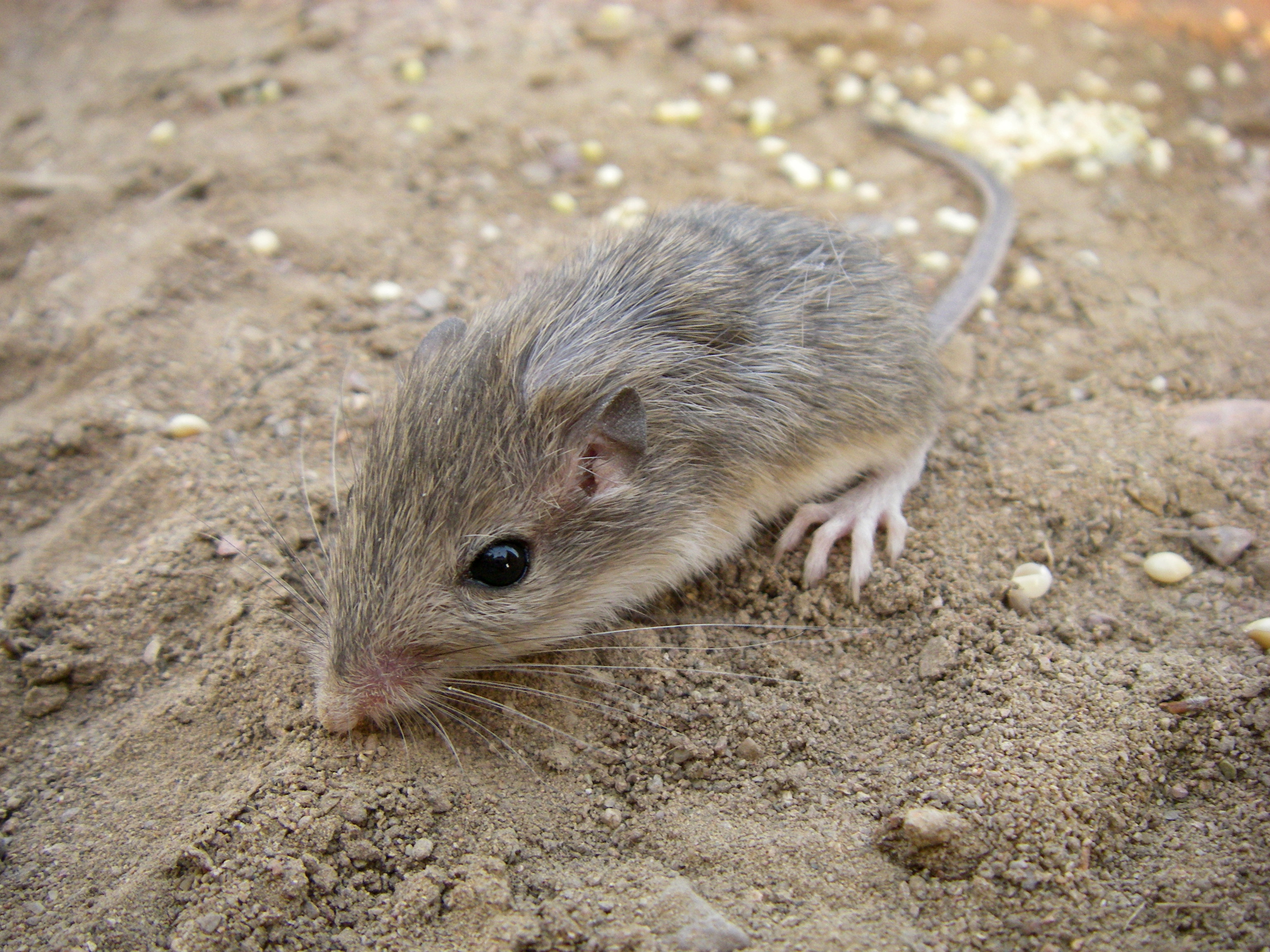
.title[
# Ecological forecasting in R
]
.subtitle[
## Lecture 1: introduction to time series models
]
.author[
### Nicholas Clark
]
.institute[
### School of Veterinary Science, University of Queensland
]
.date[
### 0900–1200 CET Monday 27th May, 2024
]

---

# Welcome

???

---
## About me
<img src="resources/NicholasClark.jpg" style="position:fixed; right:8%; top:9%; width:239px; height:326px; border:none;" />

Australian Research Council Early Career Fellow

The University of Queensland
- School of Veterinary Science 
- Located in Gatton, Australia

Expertise in:
- Quantitative ecology
- Molecular genetics
- Multivariate time series modelling

---

## Workflow

Press the "o" key on your keyboard to navigate among slides

Access the [tutorial html here](https://nicholasjclark.github.io/physalia-forecasting-course/day1/tutorial_1_physalia)
- Download the data objects and exercise `R` script from the html file
- Complete exercises and use Slack to ask questions

Relevant open-source materials include:
- [Forecasting Principles and Practice](https://otexts.com/fpp3/)
- [Applied Time Series Analysis](https://atsa-es.github.io/atsa-labs/)
- [Ecological Forecasting & Dynamics Course](https://course.naturecast.org/)
- [How to interpret nonlinear effects from GAMs](https://ecogambler.netlify.app/blog/interpreting-gams/)

---

## This lecture's topics

Why forecast?

Why are time series difficult?

Visualizing time series

Common time series models

Why they fail in ecology

---
class: inverse middle center big-subsection

# Why forecast?

---
class: middle center
###“Because all decision making is based on what will happen in the future, either under the status quo or different decision alternatives, decision making ultimately depends on forecasts”
  
[Dietze et al. 2018](https://ecoforecast.org/about/)

---

---

background-image: url('./resources/big_data.gif')
background-size: contain
background-color: #F2F2F2

---

## Where is forecasting used?
Fisheries stocks, landings and bycatch risks

Coral bleaching and algal bloom risks

Carbon stocks

Wildlife population dynamics

[Many other examples](https://ecoforecast.org/member-forecasting-profiles/)

---

## [NOAA Coastwatch's `EcoCast`](https://coastwatch.pfeg.noaa.gov/ecocast/)
.pull-right[![Ecocast system](resources/Ecocast.jpg)]
Tell fishers where to avoid bycatch

Harnesses up-to-date information for ecological models:
- Fisheries bycatch data
- Satellite observations
- Oceanography products

Builds distribution models and dynamically updates maps

---

---

## [Portal Project's `Portalcast`](https://portal.naturecast.org/)
.pull-right[<br>![Portalcast system](resources/pp_image.jpg)]

Predict rodent abundance up to one year ahead

Harnesses up-to-date information for ecological models:
- Rodent captures from baited traps
- Satellite observations

Builds time series models and dynamically update forecasts

---

background-image: url('./resources/portal_forecast.png')
background-size: contain

---

# Why are time series difficult?

---

## Some challenges of time series 
Temporal autocorrelation

Lagged effects

Non-Gaussian data and missing observations

Measurement error

Time-varying effects

Nonlinearities

Multi-series clustering

---

## Let's focus on these for now 
.emphasize[*Temporal autocorrelation*]

Measurement error

Time-varying effects

Nonlinearities

Multi-series clustering]

---

## What is temporal autocorrelation?
Values at current time .emphasize[*correlated with past values*]

`$$Cor({Y}_{t}, {Y}_{t-lag})\neq0$$`

---
## Refresher: what is correlation?

Correlation assumes a .emphasize[*linear*] relationship among two variables

---

## What is temporal autocorrelation?
Values at current time .emphasize[*correlated with past values*]

`$$Cor({Y}_{t}, {Y}_{t-lag})\neq0$$`

We can estimate the correlation `$(\beta)$` with linear regression

`$$\boldsymbol{Y}_{t}\sim \text{Normal}(\alpha + \color{darkred}{\beta} * \boldsymbol{Y}_{t-lag},\sigma)$$`

---

## What is temporal autocorrelation?
Values at current time .emphasize[*correlated with past values*]

`$$Cor({Y}_{t}, {Y}_{t-lag})\neq0$$`

We can estimate the correlation `$(\beta)$` with linear regression

`$$\boldsymbol{Y}_{t}\sim \text{Normal}(\alpha + \color{darkred}{\beta} * \boldsymbol{Y}_{t-lag},\sigma)$$`

Generalize to state that current value of a series (at time `$t$`) is .emphasize[*a function*] of it's own past values (at time `$t-lag$`)

`$$\boldsymbol{Y}_{t}\sim \text{f}( \boldsymbol{Y}_{t-lag})$$`

---
## A *positively* autocorrelated series
.panelset[
.panel[.panel-name[Code]

```r
# set seed for reproducibility
set.seed(1111)

# number of timepoints
T <- 100

# use arima.sim to simulate from an AR(1) model
series <- arima.sim(model = list(ar = 0.8), n = T, sd = 1)

# plot the time series as a line
plot(series, type = 'l', bty = 'l', lwd = 2, 
     col = 'darkred', ylab = 'Y', xlab = 'Time')
```
]

.panel[.panel-name[Model]
`$$\boldsymbol{Y}_{t}\sim \text{Normal}(\color{darkred}{0.8} * \boldsymbol{Y}_{t-1},\color{darkred}{1})$$`
]

]
]

---

## A *negatively* autocorrelated series
.panelset[
.panel[.panel-name[Code]

```r
# set seed for reproducibility
set.seed(1111)

# number of timepoints
T <- 100

# use arima.sim to simulate from an AR(1) model
series <- arima.sim(model = list(ar = -0.8), n = T, sd = 1)

# plot the time series as a line
plot(series, type = 'l', bty = 'l', lwd = 2, 
     col = 'darkred', ylab = 'Y', xlab = 'Time')
```
]

.panel[.panel-name[Model]
`$$\boldsymbol{Y}_{t}\sim \text{Normal}(\color{darkred}{-0.8} * \boldsymbol{Y}_{t-1},\color{darkred}{1})$$`
]

]
]

---
## Correlations *over >1 lag*

Can include multiple lags of the same predictor variable (the response in this case)

<br/>

`$$\boldsymbol{Y}_{t}\sim \text{f}(\boldsymbol{Y}_{t-1},\boldsymbol{Y}_{t-2},\boldsymbol{Y}_{t-3})$$`

---

## Lagged effects of predictors

External conditions (eg temperature, humidity, landcover) can also influence what happens to a series at later timepoints

<br>

`$$\boldsymbol{Y}_{t}\sim \text{f}( \boldsymbol{Y}_{t-lag}, \color{darkred}{\boldsymbol{X}_{t-lag}})$$`
<br>
Where: 
- `$\boldsymbol{X}_{t}$` is the matrix of predictor values at time `$t$`
---

class: middle center
### Many series show complex correlation structures; they can also show other temporal patterns

---

## Seasonality
.pull-right-bigger[![Lynx](resources/canada-lynx-gary-pritts.jpg)]

Many time series show .emphasize[*repeated periodic cycles*]
- Breeding seasons
- Migration
- Green-ups / green-downs
- Lunar cycles
- Predator / prey dynamics

Often change slowly over time

---

## Example seasonal series
<img src="lecture_1_slidedeck_files/figure-html/unnamed-chunk-4-1.svg" style="display: block; margin: auto;" />

---
## Another seasonal series
<img src="lecture_1_slidedeck_files/figure-html/unnamed-chunk-5-1.svg" style="display: block; margin: auto;" />
---

# Visualizing time series

---

## Detecting lagged effects
[Lag plots](https://otexts.com/fpp3/lag-plots.html)

Autocorrelation functions ([ACFs](https://otexts.com/fpp3/acf.html))

Partial autocorrelation functions ([pACFs](https://online.stat.psu.edu/stat510/lesson/2/2.2#:~:text=In%20general%2C%20a%20partial%20correlation,some%20other%20set%20of%20variables.))

Cross-correlation functions ([CCFs](https://online.stat.psu.edu/stat510/lesson/8/8.2))

---

## *Independent* correlations
.panelset[
.panel[.panel-name[Code]

```r
# set seed for reproducibility
set.seed(1111)

# number of timepoints
T <- 100

# use arima.sim to simulate from an AR(1) model
series <- arima.sim(model = list(ar = c(0.8)), n = T, sd = 1)

# plot the empirical ACF
acf(series, lwd = 2, bty = 'l',
    ci.col = 'darkred', main = '')
```
]

]
]

---

## *Conditional* correlations
.panelset[
.panel[.panel-name[Code]

```r
# set seed for reproducibility
set.seed(1111)

# number of timepoints
T <- 100

# use arima.sim to simulate from an AR(1) model
series <- arima.sim(model = list(ar = c(0.8)), n = T, sd = 1)

# plot the empirical pACF
pacf(series, lwd = 2, bty = 'l',
    ci.col = 'darkred', main = '')
```
]

]
]

---

## *Independent* cross-correlations
.panelset[
.panel[.panel-name[Code]

```r
# compute a CCF of the built-in lung cancer dataset
ccf(as.vector(mdeaths), as.vector(fdeaths), 
    # compute cross-correlations at each lag
    type = 'correlation',
    bty = 'l', lwd = 2, ci.col = 'darkred',
    ylab = "cross-correlation", main = "")
# add an informative title
title(main = expression(paste(italic(Cor),
                            "(", Female~deaths,
                            ",", Male~deaths, ")")),
          line = 0)
```
]

]
]
---

## ACFs often detect seasonality
.panelset[
.panel[.panel-name[Code]

```r
# load the 'gas' dataset from the forecast library
library(forecast)
data(gas)

# subset to the final 100 observations
gas <- gas[377:476]

# plot the empirical ACF over 48 lags
acf(gas, lag.max = 48, lwd = 2, bty = 'l',
    ci.col = 'darkred', main = '')
```
]

]
]

---
## But why did we subset?

```r
# load the 'gas' dataset from the forecast library
library(forecast)
data(gas)

# subset to the final 100 observations
*gas <- gas[377:476]

# plot the empirical ACF over 48 lags
acf(gas, lag.max = 48, lwd = 2, bty = 'l',
    ci.col = 'darkred', main = '')
```

---

## Because `gas` looks like this ...
<img src="lecture_1_slidedeck_files/figure-html/unnamed-chunk-11-1.svg" style="display: block; margin: auto;" />

---

## ... and has a nonlinear *trend*
<img src="lecture_1_slidedeck_files/figure-html/unnamed-chunk-12-1.svg" style="display: block; margin: auto;" />

---
## Raw ACF is misleading
<img src="lecture_1_slidedeck_files/figure-html/unnamed-chunk-13-1.svg" style="display: block; margin: auto;" />
---

## Decompositions
Often it is helpful to split (i.e. [decompose](https://otexts.com/fpp3/decomposition.html)) a time series into several sub-components
- Long-term trends
- Repeated seasonal patterns
- Remaining non-temporal variation

These components can be summed to give the original series

---
## Example: a complex series

---

## Decompose: trend + seasonality
<img src="lecture_1_slidedeck_files/figure-html/unnamed-chunk-15-1.svg" style="display: block; margin: auto;" />
---

## Under the hood

---

class: middle center
### Modelling these multiple components, either additively or multiplicatively, is a major goal of most time series analysis procedures

---

# Common time series models

---

## Common time series models
Random Walk ([RW](https://atsa-es.github.io/atsa-labs/sec-tslab-random-walks-rw.html))

Autoregressive ([AR](https://atsa-es.github.io/atsa-labs/sec-tslab-autoregressive-ar-models.html))

Autoregressive Integrated Moving Average ([ARIMA](https://otexts.com/fpp3/arima.html); require [stationarity](https://otexts.com/fpp3/stationarity.html))

Exponential Smoothing ([ETS](https://otexts.com/fpp3/expsmooth.html))

[Regression with ARIMA errors](https://otexts.com/fpp3/regarima.html)

---

## *Very* easy to apply in <svg aria-hidden="true" role="img" viewBox="0 0 581 512" style="height:1em;width:1.13em;vertical-align:-0.125em;margin-left:auto;margin-right:auto;font-size:inherit;fill:steelblue;overflow:visible;position:relative;"><path d="M581 226.6C581 119.1 450.9 32 290.5 32S0 119.1 0 226.6C0 322.4 103.3 402 239.4 418.1V480h99.1v-61.5c24.3-2.7 47.6-7.4 69.4-13.9L448 480h112l-67.4-113.7c54.5-35.4 88.4-84.9 88.4-139.7zm-466.8 14.5c0-73.5 98.9-133 220.8-133s211.9 40.7 211.9 133c0 50.1-26.5 85-70.3 106.4-2.4-1.6-4.7-2.9-6.4-3.7-10.2-5.2-27.8-10.5-27.8-10.5s86.6-6.4 86.6-92.7-90.6-87.9-90.6-87.9h-199V361c-74.1-21.5-125.2-67.1-125.2-119.9zm225.1 38.3v-55.6c57.8 0 87.8-6.8 87.8 27.3 0 36.5-38.2 28.3-87.8 28.3zm-.9 72.5H365c10.8 0 18.9 11.7 24 19.2-16.1 1.9-33 2.8-50.6 2.9v-22.1z"/></svg>

Hyndman’s tools in the [`forecast` 📦](https://pkg.robjhyndman.com/forecast/) are hugely popular and accessible for time series analysis / forecasting 
  
[ETS](https://pkg.robjhyndman.com/forecast/reference/ets.html) handles many types of seasonality and nonlinear trends 
  
[Regression with ARIMA errors](https://pkg.robjhyndman.com/forecast/reference/auto.arima.html) includes additive fixed effects of predictors while capturing trends and seasonality

*Some* of these algorithms can handle missing data

*All* are extremely fast to fit and forecast

---

## Great! But what about these? 
.grey[Temporal autocorrelation

Lagged effects]

*Measurement error*

*Time-varying effects*

*Nonlinearities*

*Multi-series clustering*]

---

# Time series models fail in ecology

---

## Ecological time series include
Counts of multiple species over time

Presence-absence of species

Repeated captures in multiple plots

Censored measures (OTUs / pollutants with limits of detection)

Phenology records

Tree rings

etc...

---

## Example ecological time series
</br>
.pull-left[
<img src="lecture_1_slidedeck_files/figure-html/unnamed-chunk-17-1.svg" style="display: block; margin: auto;" />
]
.pull-right[
<img src="lecture_1_slidedeck_files/figure-html/unnamed-chunk-18-1.svg" style="display: block; margin: auto;" />
]

---

## Another ecological time series
</br>
.pull-left[
<img src="lecture_1_slidedeck_files/figure-html/unnamed-chunk-19-1.svg" style="display: block; margin: auto;" />
]
.pull-right[
<img src="lecture_1_slidedeck_files/figure-html/unnamed-chunk-20-1.svg" style="display: block; margin: auto;" />
]

---

## Yet another ecological time series

</br>
.pull-left[
<img src="lecture_1_slidedeck_files/figure-html/unnamed-chunk-21-1.svg" style="display: block; margin: auto;" />
]
.pull-right[
<img src="lecture_1_slidedeck_files/figure-html/unnamed-chunk-22-1.svg" style="display: block; margin: auto;" />
]

---

## Collections of ecological series
<img src="lecture_1_slidedeck_files/figure-html/unnamed-chunk-23-1.svg" style="display: block; margin: auto;" />

---

## All can have measurement error
</br>
<img align="center" width="1200" height="300" src="resources/auger.jpg">

---

# How can we do better?

---

## In the next lecture, we will cover

Useful probability distributions for ecologists

Generalized Linear and Additive Models

Temporal random effects

Temporal residual correlation structures